Analytic, low-cost functionality from Laplace
In the previous sections, we have seen how the Laplace approximation endows a neural network with a Gaussian weight-space uncertainty (cf. Chapter Introduction to Laplace approximations), and how this uncertainty can be transformed into a closed-form expression for predictive uncertainty (cf. Chapter Linearised Laplace approximations) informed by the training data (cf. Chapter The differential geometric perspective on Laplace). By combining the linearised pushforward with analytic approximations for the softmax integral in classification, we obtain a versatile analytic toolbox for uncertainty-driven decision making.
Classical Bayesian statistical methods – such as probabilistic prediction, out-of-distribution detection, active learning, Bayesian optimisation, continual learning, and model selection – become directly accessible in deep learning under the Gaussian assumption. This setting also enables further approximations for inference at various computational budgets Daxberger et al., 2021Weber et al., 2025.
In this chapter, we examine two case studies demonstrating how such uncertainty estimates can be leveraged to address open challenges in deep learning. The first focuses on how to mitigate predictive overconfidence in ReLU networks. The second addresses continual learning: we will see that the Laplace approximation provides a natural regularisation term, which alleviates catastrophic forgetting. We then conclude with additional observations on how the Laplace-Gaussian Process connection can be leveraged for optimal data selection under different objectives. For a discussion on computational techniques for scaling these approaches to large networks, such as KFAC and subnetwork approximations, we refer to Section Scalable Curvature Approximations and Chapter Scalable Laplace approximations.
Fixing overconfidence with calibrated uncertainty
Provable overconfidence in ReLU-like neural networks
In supervised classification, deep neural networks are trained to map an input to a vector of class logits , which are converted into categorical probabilities via the softmax function (57). Ideally, these probabilities should reflect the true uncertainty of the model’s predictions. In practice, however, modern deep networks tend to be overconfident: they assign very high probabilities to certain classes even when the input is far from the training distribution. This behaviour is particularly problematic in safety-critical settings, such as medical diagnosis or autonomous driving, where unwarranted certainty can have serious consequences Hein et al., 2019.
A precise theoretical explanation for this behaviour in ReLU-like networks was given by Hein et al. (2019). Such networks consist of linear layers (fully connected or convolutional) combined with piecewise-linear activations such as ReLU or LeakyReLU. Consequently, they implement a piecewise affine mapping:
where the polytopes partition the input space into regions of constant activation pattern. Within each such region, the logits grow linearly with . As the input moves far away from the training data, the behaviour is dominated by a single affine component whose largest logit can grow without bound, while all other logits remain comparatively smaller. Since the softmax function magnifies differences between logits, this causes the predicted probability for a single class to approach one.
In other words, deterministic ReLU networks extrapolate with increasing certainty as we move away from training data, regardless of the lack of evidence.
Bayesian perspective as a counter measure
The problem identified in the previous section is an artefact directly caused by the use of point estimates. The natural way to solve it is to assign a probability measure over the weights instead of committing to a single value. As we will see, this naturally leads to increasing variance away from the data, which tempers the confidence after the softmax is applied.
The Laplace approximation provides a tractable route to introduce this behaviour into neural networks. To recall, we approximate for a given trained network with parameters (the maximum a posteriori estimate), the posterior over parameters by a Gaussian:
where describes the curvature of the negative log posterior evaluated at . With linearising the pushforward around , the logits become Gaussian as well (cf. Section Linearisation):
with
For ReLU networks, the components of grow at most linearly with , so the logit variance grows quadratically with (equivalently, the standard deviation grows linearly). This means that, far from the training set, the variance in each logit matches the mean’s linear growth. We will now see that this leads to finite asymptotic confidence in each class, bounded away from 1 and 0.
The predictive class probabilities are obtained by marginalising over the Gaussian posterior
While exact evaluation is infeasible, accurate analytic approximations exist (cf. Section The Predictive). A well-known approximation in the binary case is due to MacKay (1992):
where is the Gaussian logit with mean and variance , and is the logistic sigmoid.
This solution was established by Kristiadi et al. (2020) in their paper Being Bayesian, Even Just A Bit, Fixes Overconfidence In ReLU Networks, where Even Just A Bit refers to the observation that the following theorem holds even when only the weights of the last layer are treated probabilistically, and even if the covariance in the Laplace approximation is chosen in an arbitrary way (say, equal to the identity ).
Here, denotes the largest eigenvalue of the negative log-likelihood Hessian evaluated at the posterior mean , while and are the mean logit and network Jacobian at , exactly as in Equation (6). Note that differs from the posterior precision only by the Gaussian-prior term, , and this prior contribution vanishes as , so only the likelihood Hessian survives in the bound.
Of course, this theorem provides only an asymptotic statement. In words: If we assign any Gaussian measure to the weights of the network (whether explicitly constructed as a Laplace approximation or simply imposed) then asymptotic overconfidence is “healed” in the weak sense that it is bounded away from 1 and 0. Despite its weak form, this result is a great argument for balancing the cost of Laplace approximations with their goals. If all you want is to fix asymptotic confidence, then you can do so at virtually zero computational cost: Just impose an arbitrary confidence on the parameters. This is still better than using a point estimate instead.
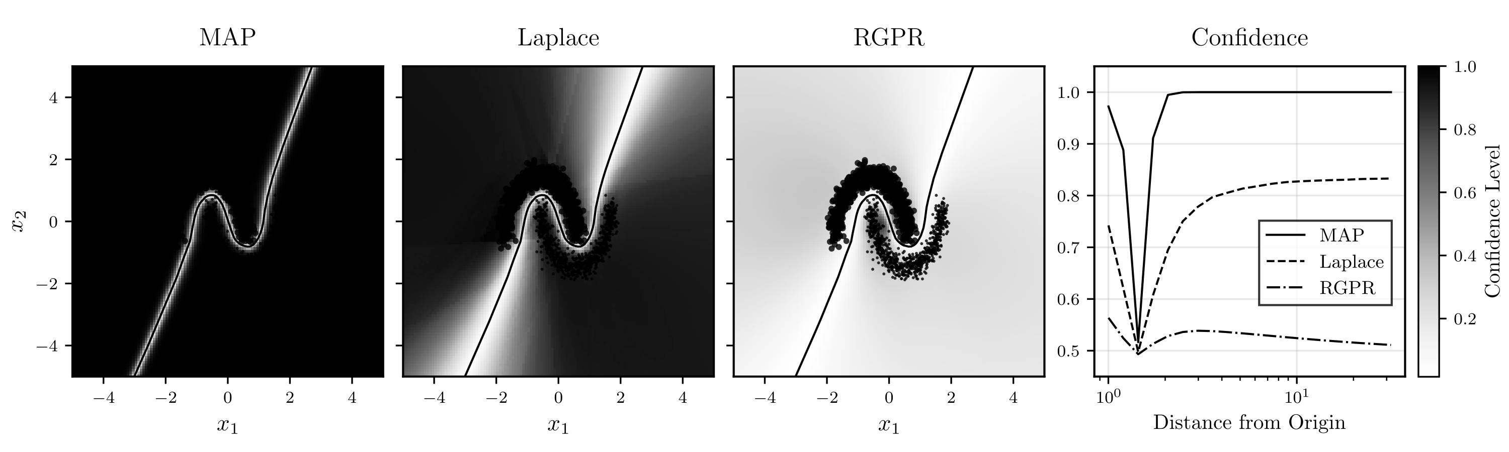
Figure 1:Mitigating overconfidence in a ReLU network with the Laplace approximation. The figure shows the predictive confidence on a two-moons binary classification task for three different models. Darker background shading indicates higher confidence, while the solid black line marks the decision boundary at . (Left) The standard MAP-trained ReLU network exhibits severe overconfidence. As described in Theorem 1, its predictive confidence incorrectly approaches 1 (maximum certainty) for inputs far away from the training data. (Middle) Applying the Laplace approximation introduces uncertainty over the network’s weights. The resulting logit variance grows quadratically with distance from the data, which tempers the softmax and reduces predictive confidence in out-of-distribution regions. (Right) Adding a ReLU-GP residual term (RGPR) to the Laplace-approximated logits introduces an additional source of variance that grows cubically. This ensures that the predictive confidence correctly converges to the uniform distribution (0.5) for inputs far from the training data, providing better calibration. (Far Right) This panel quantitatively confirms the visual results by plotting the maximum confidence of each model as an input point is scaled away from the origin.
The role of the prior variance
Theorem 2 highlights the special role of the prior variance : increasing broadens the posterior over weights, which in turn accelerates variance growth in the logits and reduces predictive confidence away from the data. On the other hand, letting recovers the deterministic prediction. Although is traditionally motivated by the weight decay used during training, in the Laplace setting it can be tuned post hoc to improve the calibration.
Hyperparameters such as the prior variance or additional factors entering the curvature can be tuned with techniques often motivated by the literature on Gaussian processes Rasmussen & Williams, 2006. This includes downstream objectives (e.g., negative log-likelihood, out-of-distribution entropy) or model fit criteria (e.g. log marginal likelihood). Here, the Gaussian structure of the Laplace approximation allows for closed-form objectives suitable for gradient-based tuning, which is discussed in more detail in addition to other applications in the next chapter (cf. Chapter Model selection with the marginal likelihood).
For the particular setting of calibrating such that the resulting uncertainty structure reflects out-of-distribution well, Kristiadi et al. (2020) suggest using
where the first term is the standard cross-entropy loss over an in-distribution validation set , while the second is the predictive entropy over a set of out-of-distribution inputs , which the objective encourages to be large through the leading minus sign. The parameter controls the trade-off between these two terms.
How to mitigate the problem even further
A simplified summary of Theorem 2 is that assigning a Gaussian measure to weights bounds asymptotic confidence away from the pathological values 1 and 0. But it will not drive asymptotic confidence down to the ideal uniform (maximum entropy) limit where is the number of classes. And of course the Theorem says nothing about confidence “close to” or “in-between” the training data. To address either problem, Kristiadi et al. (2021)Kristiadi et al. (2021) consider two extensions to tune the overall confidence structure: one reshapes the local curvature for better calibration close to the data Kristiadi et al., 2021, the other combines the weight-space uncertainty with some additional output-space uncertainty to ensure the ideal uniform confidence limit Kristiadi et al., 2021.
The approach Learnable Uncertainty under Laplace approximations (LULA) Kristiadi et al., 2021 augments a trained network with additional parameters – uncertainty units – inserted into the architecture in a way that preserves the MAP prediction but modifies the Hessian , e.g. for three linear layers without nonlinearities and biases for simplicity, we have,
Therefore, the final variance changes while the mean prediction stays the same, which motivates the name uncertainty units. These units are then trained using an uncertainty-aware loss that encourages high predictive entropy on out-of-distribution (OOD) inputs and low entropy on in-distribution (ID) inputs, with gradients masked so that the original prediction remains unchanged. It can then be shown that the resulting Laplace approximation with diagonal curvature approximation has higher variance over the output compared to the diagonal Laplace for the network without the uncertainty units (cf. Proposition 2, Kristiadi et al. (2021)).
However, residual overconfidence can still be left for inputs extremely far from the training data. This is a consequence of the fact that ReLU networks have only finitely many effective features, whereas a Gaussian process (GP) with an infinite set of ReLU features exhibits a growth of cubic variance, forcing the softmax confidence toward the uniform distribution as . The ReLU-GP residual (RGPR) approach Kristiadi et al., 2021 adds such a GP as an independent residual term to the Bayesian neural network:
with a specific double-sided cubic spline kernel chosen so that near the origin but grows cubically with . The resulting logit distribution is
preserving the mean while adding variance that dominates in the tails. Applying a softmax approximation to this Gaussian results in a predictive distribution that converges to the uniform distribution in the limit (cf. Theorem 4, Kristiadi et al. (2021)).
Importantly, this Gaussian process term can be added in such a way that its evaluation has constant and negligible cost, independent of the training data. This is because it is explicitly constructed to not be affected by data within the training region, only contributing prior uncertainty in the OOD regime. It is thus another example of a Laplace approximation adding specific functionality, at extremely minimal cost overhead. The double-sided cubic spline kernel chosen in this work also has a pleasing interpretation as a limit process arising from an infinite number of the ReLU uncertainty units from above, all distributed in a regular fashion around the training domain, pointing “outwards” so that they are not affected by the training data. The implied intuition is that these units “complete” or complement the finitely many ReLUs that make up the deep network that we actually train on the available (finite) data, and provide a nonparametric sea of ReLUs that cover the domain towards the horizon. To speak even more metaphorically, this is arguably an example of the Bayesian perspective on deep learning providing an intuition – and a concrete, practical solution! – to a pathology of point-estimated deep models. Figure 1 compares the predictive confidence of the MAP network, its Laplace approximation, and the RGPR extension on a two-moons task, illustrating how each successive step tempers overconfidence away from the data.
Fixing catastrophic forgetting in continual learning
In continual learning, a single neural network is trained on a sequence of tasks
with the goal of maintaining good performance on earlier tasks. This setting is increasingly relevant in real-world deployments: modern large-scale models are trained once, but are then confronted with a stream of evolving data and objectives. A key obstacle to adaptation is catastrophic forgetting, the loss of previously acquired abilities when learning new tasks.
A naïve approach is to fine-tune the current parameters by minimising the loss on the next dataset :
However, this discards all information about earlier tasks: parameters drift toward the new optimum for adapting to the new data , and end up erasing information by neglecting critical weights for previous performance.
A Bayesian solution
From a Bayesian perspective, training on should not start from an uninformative prior. Instead, the posterior after task should become the prior for task :
instead of the original uninformative isotropic Gaussian in form of weight decay. Taking the negative log turns this into a regularised optimisation problem, where the regulariser encodes knowledge from earlier tasks.
If is approximated by a Gaussian via the Laplace approximation Sliwa et al., 2024, the next-task objective becomes:
where denotes the squared Mahalanobis norm induced by the precision . The precision matrix determines how strongly each direction in parameter space is protected: large precision (high curvature) means a stiff penalty in that direction, since the loss on the previous task would change rapidly, while low precision allows for adaptation. This yields an anisotropic weight-space prior that selectively resists change where it would harm past performance. The regularisation strength controls the trade-off between retaining performance on past tasks and adapting to new ones by scaling the precision of the prior: higher values express greater confidence in past parameters, lower values signal greater uncertainty and openness to change.
Bayesian filtering in weight space
Starting from the previously motivated interpretation and following Sliwa et al. (2024), we can formalise continual learning as Bayesian state estimation in weight space:
with a Gaussian state-transition model and a likelihood defined by the task loss
Continual learning becomes in this interpretation a problem of tracking a moving target in weight space: the process model predicts where the target might go next, and the observation model corrects this prediction based on new evidence. The additional process noise covariance models the expected drift between tasks: large corresponds to high plasticity (parameters may change substantially), while small enforces stability (parameters remain close).
The Bayesian filtering recursion consists of:
Predict step: propagate the posterior through the process model to obtain a prior for , (potentially) inflating the uncertainty by .
Update step: incorporate the likelihood from , pulling the mean toward the new optimum and shrinking uncertainty according to curvature.
This is analogous to a Kalman filter in parameter space, but with a nonlinear, non-Gaussian observation model arising from the neural network loss. The Laplace approximation replaces this intractable term with a local Gaussian, making the update step analytically tractable within the filtering framework.
From EWC to OSLA to Lo-Fi
The state-space formulation provides a unifying Bayesian view of continual learning. Different methods in the literature can be seen as specific choices for (i) how the posterior covariance is represented and updated, and (ii) whether parameter drift between tasks is allowed. The Laplace approximation supplies the Gaussian form needed for tractable updates, but the quality and scalability of the approach depend on the curvature approximation used.
Elastic Weight Consolidation (EWC).
Kirkpatrick et al. (2017) proposed elastic weight consolidation (EWC), which constrains parameters to remain close to the previous optimum using the diagonal of the Fisher information metric :
This is equivalent to the proposed filtering framework when choosing and a diagonal precision. In the sequential setting, a separate quadratic penalty can be added for each of the previous tasks (multi-penalty), or equivalently, the Fisher matrices can be accumulated into a single continuously updated penalty. EWC is computationally efficient but lacks correlation between parameters.
Online Structured Laplace Approximation (OSLA).
Ritter et al. (2018) extended EWC by replacing the diagonal Fisher with a Kronecker-factored (KFAC) curvature approximation (cf. Section Scalable Curvature Approximations), capturing intra-layer parameter correlations while remaining scalable. In the Bayesian filtering view, OSLA maintains a single Gaussian posterior over parameters and updates it recursively after each task:
where is again the Fisher information matrix computed with the current MAP estimate on task . The running update replaces the need to store separate penalties for each task, as in multi-penalty EWC, and naturally implements a sequential Bayesian update with (no assumed drift). By incorporating inner-layer correlations, OSLA produces a more faithful posterior approximation and better retention over long sequences of tasks.
Low-Rank Laplace-Gaussian Filtering (Lo-Fi).
Chang et al. (2023) and Sliwa et al. (2024) generalised the Bayesian framework to arbitrary , enabling explicit modelling of expected drifts between tasks. They approximate the precision matrix using a low-rank approximation of the GGN (plus diagonal representing the initial prior), which makes both, prediction and update step, scalable while still modelling correlation between different layers.
In this general Bayesian filtering view, the concept of smoothing also becomes available. After the forward filtering pass, an optional backward pass refines each task-specific parameter estimate using information from future tasks without revisiting their original data. The process can be compared to passing a message along a chain of messengers, where each messenger (task) has access only to the message (parameters) they just received and their own local observations; over time, the message can degrade (catastrophic forgetting). Smoothing allows later messengers to send clarifications or corrections back upstream, improving earlier versions without re-reading the original letters (data). In a deep learning context, this means earlier task models can be improved based on knowledge from later tasks, while preserving data privacy by never sharing or replaying the original datasets from other tasks.
Data-centric objectives
The Laplace approximation provides a tractable way to understand the relationship between a model and its training data, which, in turn, improves properties such as predictive calibration (cf. Section Fixing overconfidence with calibrated uncertainty) and the ability to learn sequentially (cf. Section Fixing catastrophic forgetting in continual learning). The same model-data relationship is central to the fields studying optimal data selection. Rather than relying on random sampling, methods have been developed to strategically choose the most informative data to label (active learning) and the most efficient points to evaluate (Bayesian optimisation). A fundamentally Bayesian approach underpins these strategies, leveraging a model’s current beliefs to guide data acquisition. Also more nuanced data-centric questions exist, such as determining the most effective training order (curriculum learning), that have been studied from a Bayesian perspective with the help of the Laplace approximation Deng et al., 2023. However, here, we focus on active learning and Bayesian optimisation due to their foundational connection to Bayesian principles.
Active learning: selecting what to label next
The goal of active learning is to train an optimal model with a minimal data collection effort. For instance, training neural solvers for partial differential equations often requires a vast amount of training data generated by costly numerical simulations. Instead of random generation, active learning aims to strategically select the most informative data points to label, thereby achieving the same model accuracy with significantly less numerical simulations Musekamp et al., 2025.
From a Bayesian perspective, this selection process can be formalised as an optimisation problem guided by information theory. MacKay (1992) proposed framing active learning as a sequential design task where the goal is to choose the next data point that is expected to provide the maximal information gain about the model’s parameters . This gain is measured by the expected reduction in the entropy of the parameter posterior after observing a new data point :
where denotes the (differential) entropy of a distribution ; for a discrete distribution, such as the class-label predictive , the integral is replaced by the sum .
In general, computing this expected information gain is intractable, though the linearised Laplace approximation provides again a solution. By approximating the posterior with a Gaussian, MacKay (1992) showed that the expected information gain from a potential new data point at input is a monotonic function of the model’s current predictive variance at that location . This provides a principled justification for the intuitive and widely used uncertainty sampling heuristic: to learn the most, one should query the points where the model is currently most uncertain MacKay, 1992.
The objective of maximising parameter information is now widely known as Bayesian Active Learning by Disagreement (BALD) Houlsby et al., 2011. The BALD score is a mathematically equivalent reformulation of the original objective:
This version provides the powerful intuition that one should query points where the model is overall uncertain about its prediction (the first term), but where individual parameters from the posterior are confident in their potentially disagreeing predictions (the second term is low).
It has been observed, that BALD’s focus on parameter uncertainty can be misaligned with the goal of predictive performance, as it lacks an explicit notion of the relevant input data distribution. This can lead to the selection of obscure or irrelevant data points that offer little benefit to typical test input. To address these shortcomings, the Expected Predictive Information Gain (EPIG) Mindermann et al., 2022 was proposed, which measures the expected information a candidate label at input provides about the label of a random target input drawn from a target distribution . This objective is formalised as the expected reduction in predictive entropy on a random target point, averaged over all possible outcomes of the candidate query:
Both the BALD and EPIG objectives are agnostic to the method used for posterior approximation. By shifting the entropy computation to the lower-dimensional prediction space (BALD) or considering only the predictive entropy (EPIG), this information-theoretic approach lessens the reliance on a specific form of weight-space uncertainty, opening the door for various uncertainty quantification tools. The Laplace approximation remains a fast and tractable method for obtaining the predictive uncertainty needed to compute either score. Ultimately, however, the performance of these acquisition functions is strongly coupled to the quality of the resulting uncertainty estimates.
Bayesian optimisation: finding the optimal point
Many problems can be framed as finding the global optimum of an objective function that is very expensive to evaluate. Bayesian optimisation (BO) is a sequential strategy for finding the global optimum of such expensive black-box functions and works by combining a probabilistic surrogate model of the objective with acquisition functions to select the next point for evaluation Garnett, 2023. Gaussian Processes (GPs) are the standard surrogate model because they are inherently Bayesian, providing a posterior distribution over the function and allowing for many popular acquisition functions to be computed analytically, making the entire process efficient and principled.
The linearised Laplace approximation (LLA) provides a way of using neural networks as surrogates by interpreting them as a Gaussian Process, which allows for reusing existing analytic acquisition functions, such as maximising the upper confidence bound given by
where is the network’s mean prediction at the MAP estimate, is the predictive standard deviation from the LLA posterior and a hyperparameter balancing exploration and exploitation Kristiadi et al., 2023.
The final optimisation process is then iterative. At each step, a neural network is trained on the existing data set and queried using the LLA and an acquisition function for the next data point to evaluate the original black-box function. Then, this new information must be incorporated by retraining or adapting the neural network on the augmented dataset to find a new maximum-a-posteriori (MAP) estimate and then re-computing the Laplace approximation around this new point. This refines the model’s beliefs and its weight-space uncertainty, guiding the next decision in the sequence.
Kristiadi et al. (2023) demonstrated that the LLA surrogate inherits the strong predictive power and inductive biases of its underlying neural network, allowing it to outperform standard GPs on complex, high-dimensional tasks like searching through image spaces. However, they also note that broken predictive behaviour in extrapolation regions can significantly derail the optimisation process. This becomes clear when considering the Upper Confidence Bound as an example. For a ReLU network, the predictive mean outside the data region becomes a non-constant linear function. This means the predicted value will increase or decrease indefinitely as you move away from the data, while the uncertainty term also tends to grow linearly in these extrapolation regions, following the discussion in Section Bayesian perspective as a counter measure. Since both terms grow linearly, and the UCB score uses their sum, this utility also increases without bound in the same direction, leading the optimiser to choose a point infinitely far away in an unbounded search space. Note that this behaviour is consistent within the context of UCB: A region of extremely large expected reward and extremely large uncertainty is a very appealing target for another experiment. So the problem here is arguably not the Bayesian treatment, but a badly chosen model class. Namely one that quite literally believes in pots of gold at the end of the rainbow.
- Daxberger, E., Kristiadi, A., Immer, A., Eschenhagen, R., Bauer, M., & Hennig, P. (2021). Laplace Redux - Effortless Bayesian Deep Learning. In M. Ranzato, A. Beygelzimer, Y. Dauphin, P. S. Liang, & J. W. Vaughan (Eds.), Advances in Neural Information Processing Systems (Vol. 34, pp. 20089–20103). Curran Associates, Inc.
- Weber, T., Mucsányi, B., Rommel, L., Christie, T., Kasüschke, L., Pförtner, M., & Hennig, P. (2025). laplax - Laplace Approximations with JAX. Championing Open-Source DEvelopment in ML Workshop \@ ICML25.
- Hein, M., Andriushchenko, M., & Bitterwolf, J. (2019). Why ReLU Networks Yield High-Confidence Predictions Far Away From the Training Data and How to Mitigate the Problem. IEEE/CVF Conference on Computer Vision and Pattern Recognition (CVPR).
- MacKay, D. J. C. (1992). The Evidence Framework Applied to Classification Networks. Neural Computation, 4(5), 720–736.
- Kristiadi, A., Hein, M., & Hennig, P. (2020). Being Bayesian, Even Just a Bit, Fixes Overconfidence in ReLU Networks. In H. D. III & A. Singh (Eds.), Proceedings of the 37th International Conference on Machine Learning (Vol. 119, pp. 5436–5446). PMLR.
- Rasmussen, C. E., & Williams, C. K. I. (2006). Gaussian Processes for Machine Learning. The MIT Press.
- Kristiadi, A., Hein, M., & Hennig, P. (2021). Learnable uncertainty under Laplace approximations. In C. de Campos & M. H. Maathuis (Eds.), Proceedings of the Thirty-Seventh Conference on Uncertainty in Artificial Intelligence (Vol. 161, pp. 344–353). PMLR.
- Kristiadi, A., Hein, M., & Hennig, P. (2021). An Infinite-Feature Extension for Bayesian ReLU Nets That Fixes Their Asymptotic Overconfidence. In M. Ranzato, A. Beygelzimer, Y. Dauphin, P. S. Liang, & J. W. Vaughan (Eds.), Advances in Neural Information Processing Systems (Vol. 34, pp. 18789–18800). Curran Associates, Inc.
- Sliwa, J., Schneider, F., Bosch, N., Kristiadi, A., & Hennig, P. (2024). Low-Rank Filtering and Smoothing for Sequential Deep Learning.
- Kirkpatrick, J., Pascanu, R., Rabinowitz, N., Veness, J., Desjardins, G., Rusu, A. A., Milan, K., Quan, J., Ramalho, T., Grabska-Barwinska, A., Hassabis, D., Clopath, C., Kumaran, D., & Raia Hadsell. (2017). Overcoming catastrophic forgetting in neural networks. Proceedings of the National Academy of Sciences, 114(13), 3521–3526.
- Ritter, H., Botev, A., & Barber, D. (2018). Online Structured Laplace Approximations for Overcoming Catastrophic Forgetting. In S. Bengio, H. Wallach, H. Larochelle, K. Grauman, N. Cesa-Bianchi, & R. Garnett (Eds.), Advances in Neural Information Processing Systems (Vol. 31). Curran Associates, Inc.
- Chang, P. G., Durán-Martín, G., Shestopaloff, A., Jones, M., & Murphy, K. P. (2023). Low-rank extended Kalman filtering for online learning of neural networks from streaming data. In S. Chandar, R. Pascanu, H. Sedghi, & D. Precup (Eds.), Proceedings of The 2nd Conference on Lifelong Learning Agents (Vol. 232, pp. 1025–1071). PMLR.
- Deng, Z., Cui, P., & Zhu, J. (2023). Towards Accelerated Model Training via Bayesian Data Selection. In A. Oh, T. Naumann, A. Globerson, K. Saenko, M. Hardt, & S. Levine (Eds.), Advances in Neural Information Processing Systems (Vol. 36, pp. 8513–8527). Curran Associates, Inc.
- Musekamp, D., Kalimuthu, M., Holzmüller, D., Takamoto, M., & Niepert, M. (2025). Active Learning for Neural PDE Solvers. In Y. Yue, A. Garg, N. Peng, F. Sha, & R. Yu (Eds.), International Conference on Learning Representations (Vol. 2025, pp. 38777–38825).
- MacKay, D. J. C. (1992). Information-Based Objective Functions for Active Data Selection. Neural Computation, 4(4), 590–604.