Model selection with the marginal likelihood
The main intractability of high-dimensional Bayesian inference, as mentioned earlier in the book, stems from the difficulty of computing the normalising constant of the posterior distribution—the marginal likelihood (or evidence). While the MCMC methods presented before circumvent this problem by allowing us to sample from an unnormalised posterior distribution, the Laplace approximation offers the benefit that we can compute this quantity in closed form due to the Gaussianity. This not only enables inference and predictions (as shown in the previous chapters), but has one additional important use case: model selection. In this chapter, we will motivate why the marginal likelihood is a useful model selection criterion, explain how it is computed with the Laplace approximation, and present several practical use cases for model selection in Bayesian deep learning.
Marginal likelihood for model selection
There are several perspectives to understand why the marginal likelihood can be a useful criterion for model selection. We will review some different ones in this section to hopefully convince you that this pesky normalisation constant is not only a nuisance but a powerful tool when wielded in the right way.
Hierarchical Bayes
Let us look at the familiar Bayes’ rule, but with an explicit conditioning on our model of choice, which we will denote by . This model can encompass both the prior and the likelihood, so in the case of Bayesian deep learning, for instance, the neural network architecture, the likelihood noise level, the prior variance, or its distributional form. In short, the model contains everything we have to choose actively before we can start to perform inference. The model-conditioned Bayes’ rule looks like this:
If we assume now that we do not actually know how to select the model in advance and would like to be Bayesian about it, we could attempt to treat as a random variable in a hierarchical Bayesian model, the posterior of which would take the form
If we further assume that a priori, we do not have any preference for any particular model, that is, is uniform across models (brushing under the rug the fact that this may be an improper prior if the space of models is not integrable), this yields
We now see that the hierarchical posterior over models is proportional to the marginal likelihood term in Equation (1). Therefore, if we want to select the model that maximises the posterior (i.e., a MAP estimate over models), we just need to optimise with respect to the marginal likelihood! Since this is essentially just performing a maximum likelihood selection on the second level of this Bayesian hierarchy, it is also often called maximum likelihood II (ML-II) model selection.
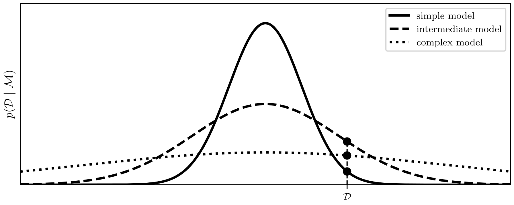
Figure 1:A visualisation of the Occam’s razor effect of the marginal likelihood. The simplest model can assign the largest likelihoods, but just to a small number of datasets. For the most complex model, it is the other way around. For a given dataset , the marginal likelihood selects an intermediate model that is just complex enough to model these data.
Occam’s razor
Apart from the interpretation as maximum likelihood in a hierarchical Bayesian model, we can also motivate from first principles why the marginal likelihood as a model selection criterion leads to an automatic Occam’s razor effect. The principle of Occam’s razor states that among a set of hypotheses (or models) that explain the same data equally well, one should always prefer the simplest one Sober, 2015. The connection to the marginal likelihood has already been made in David MacKay’s popular textbook MacKay, 2003, based on his thesis Mackay, 1992, and has been further developed by Rasmussen & Ghahramani (2000).
The argument is relatively simple: since the term has to be a normalised distribution over all possible datasets for any given model , this means that models can either assign a lot of likelihood to a small number of datasets or a small amount of likelihood to many datasets. The former would intuitively be a simple model, such as a linear one, whereas the latter would be a complex model, such as a large neural network. For a dataset that can be modelled well by a linear function, the linear model will therefore be able to assign a larger likelihood than the neural network, because its likelihood is not distributed over all the non-linear datasets. Generally, this means that the model with the largest marginal likelihood for a given dataset will typically be a model that is just complex enough to model this dataset, but not more complex, thus implementing Occam’s razor. This intuition is visualised in Figure 1.
Cross-validation
A popular non-Bayesian model selection criterion is cross-validation. The idea is that you split your dataset into , with disjoint training and validation sets and . We can then estimate the generalisation risk (i.e., the expected loss on unseen data) by training a model on and then evaluating its error on . This fits the intuition that we are ultimately interested in applying our model to unseen test data , so we want to know how well the model predicts on datapoints it has not seen during training.
In their seminal paper, Fong & Holmes (2020) show that the log marginal likelihood on is equal to the average validation log likelihood over all possible cross-validation splits, that is,
where is a shorthand for writing a mechanism that first uniformly samples a dataset size split and then samples a uniformly random permutation of assigning points to and points to . Note that for notational convenience, we have suppressed the explicit conditioning on , but you can indeed read all the here as implicitly being .
Obviously, actually performing this exhaustive cross-validation procedure would require a computational cost scaling combinatorially with the dataset size , so nobody would actually compute this in practice. However, we see that with the marginal likelihood, we get the result of this exhaustive procedure by solving just a single integral over the training dataset. This is another argument for the marginal likelihood as a model selection criterion: if you believe that cross-validation is a good way to evaluate the potential generalisation capabilities of your model, the marginal likelihood will not only compute one cross-validation for you, but all of them at the same time!
PAC-Bayes
Another way to study the generalisation behaviour of Bayesian predictors is to use the framework of PAC-Bayes bounds Shawe-Taylor & Williamson, 1997McAllester, 1998. While we will get a more thorough introduction to PAC-Bayes bounds in later chapters (specifically in Chapter PAC-Bayesian deep neural network ensembles), for now it suffices to say that they are mathematical statements that bound the expected true risk of our (approximate) posterior—which we cannot know because we do not have access to the true data-generating process—with the expected empirical risk that we can actually measure. These bounds generically look something like this:
Here, is a term that measures the model complexity. In a simple case, this could, for instance, be McAllester, 1998Pérez-Ortiz et al., 2021
This bound fits several key intuitions: it gets tighter as the size of the dataset grows because the model can overfit less; it gets looser if we reduce because then the bound needs to hold with higher probability; and it gets looser as the KL-divergence between posterior and prior grows because then the model can overfit more.
In summary, to get a small bound on the expected risk, you need a posterior that predicts well in terms of empirical risk and at the same time is as simple as possible in terms of the complexity measure . If this again sounds like Occam’s razor to you, you will not be surprised to learn that PAC-Bayes bounds can be formally connected to the marginal likelihood (indeed, this section would probably not be part of this chapter otherwise).
If we take the posterior in the bound to be the true Bayes posterior, Germain et al. (2016) derive the following PAC-Bayes bound. Note that the true posterior is often intractable and can only be approximated, in which case the bound will only hold approximately. Note also that it only holds under the technical condition that the log likelihood is sub-Gamma; a sub-Gamma loss is one whose tails are upper-bounded by the tails of a Gamma distribution, essentially ensuring that the loss does not grow unexpectedly fast. This holds, for instance, for Bayesian linear regression with a Gaussian likelihood.
We therefore see that maximising the marginal likelihood directly minimises this bound on the generalisation error, providing another strong (frequentist) argument for why it is a reasonable criterion for model selection. Remember, however, as a caveat, that this result only strictly holds for sub-Gamma likelihoods, such as for linearised Laplace in the regression setting, but not in the case of full Laplace inference in BNNs, especially in the classification setting. For those cases, the bound does not provide a proper guarantee, but still an intuitive argument for why the Occam’s razor effect of the marginal likelihood can improve generalisation.
Differentiable marginal likelihood with Laplace
So now that we have convinced ourselves that the marginal likelihood is a great criterion for model selection, we are left with the problem of actually computing (or approximating) it. Indeed, this is one of the main challenges of Bayesian inference, which is why, in practice, the marginal likelihood is not often used for this purpose. However, as promised above, the Laplace approximation has the lucky property that we can actually compute the marginal likelihood in closed form!
To understand how we can do that, we will need to look under the hood of the Laplace approximation in Equation (5). Let us remind ourselves that we are aiming to approximate the posterior
where we have now written the unnormalised posterior as . In the context of model selection, feel free to mentally condition all of these distributions on as in Equation (1) above. We will omit this conditioning here to not needlessly clutter the notation. Note also that we can choose the regularised risk from Equation (2) to be .
If we approximate around a point , this gives
where is the same Hessian operator as in Equation (7). Note that is the Hessian of , hence the sign change in the Taylor expansion.
If we now choose to be a maximiser of the (log) posterior, such that the first-order term vanishes because , and ignore the third and higher order terms, we can approximate with a distribution , which we define as
Now, instead of computing the true marginal likelihood , we can just approximate it with the normaliser of our approximate distribution, that is .
Since we see from the quadratic form in the exponential that is multivariate Gaussian with mean and precision matrix , we can look up the normalising constant, which is , where is the dimensionality of the parameter space. This means that . Therefore, our approximate log marginal likelihood is
Note that in the last line, we assumed that the number of parameters is the same across the different models that are being compared. If the model selection is meant to be performed across models with different numbers of parameters, this term naturally is not constant and still needs to be considered in the marginal likelihood.
Computational considerations
Similar to the inversion discussed in previous chapters, the determinant also has a computational cost of if the matrix is of size . As discussed before, this can get very expensive when the dimensionality of the parameter space is large, that is, for large neural network models. However, luckily, we can use some computational tricks and approximations to reduce the computational cost, such as linearisation and the empirical Fisher information, as well as diagonal or low-rank approximations (see Chapter Linearised Laplace approximations and Chapter Scalable Laplace approximations for details). Since none of these considerations are unique to the marginal likelihood computation, we will not discuss them at length in this chapter.
Post-hoc vs. online model selection
When selecting models using the marginal likelihood, the most naïve way is to perform post-hoc model selection. For instance, we can train two models, and , and then compute their respective (log) marginal likelihoods. For illustration purposes, let us say that is a fully-connected neural network and is a convolutional neural network. We train them both on some image dataset (e.g., MNIST) and then compute . If this quantity is positive, we select , if it is negative, we select . Note that this difference between log marginal likelihoods is equivalent to the likelihood ratio test, which, according to the famous Neyman-Pearson lemma Neyman & Pearson, 1933, is the uniformly most powerful hypothesis test.
This selection approach gives us all the benefits of the marginal likelihood described in the previous section, but it still requires that we train each of the different models we want to test. Indeed, for selecting some parts of the model, we can do much better than that! While the neural network architecture is a discrete choice that we have to test post hoc, there are hyperparameters of the neural network with respect to which we can actually compute gradients of the marginal likelihood and then optimise them online. These include, for instance, the variance(s) of the prior or the likelihood noise. We will denote as the subset of parameters for which gradients exist. We can then optimise these parameters by performing simple gradient ascent like
where is a step size. This allows us to select all these model hyperparameters within a single training run, without the need to train several models, as would be the case for approaches such as cross-validation.
However, this approach comes with a few caveats: First, recall that the marginal likelihood depends on the Hessian , so on the second derivatives of the loss. If we want to take gradients of the marginal likelihood, we need to ensure that these are differentiable with respect to the hyperparameters, which is not true for all activation functions. Particularly, it is not true for the ReLU activation function, so we need to ensure to use smoother ones if we want to perform online model selection (e.g., sigmoid, tanh, Swish, GeLU, ELU, etc.). Second, since the marginal likelihood depends on the entire dataset , computing it requires an entire pass over the dataset, so in deep-learning parlance, one epoch. Since the best parameters generally depend on the choice of , we typically interleave the training, that is, we train for one or more epochs and then make one or several gradient steps on the marginal likelihood as written above, each of which corresponds to an additional epoch on the data. Depending on the frequency of these updates, the training will therefore require more epochs; in practice, typically around twice as many. Finally, dropping the first-order term in the Taylor expansion above required to be a true optimum of the loss, where the gradients vanish, but one might wonder whether standard optimisers actually find such optima in deep learning. Indeed, in practice, the optima we find do not truly have zero gradients everywhere. However, it has been shown empirically that this generally does not impair the model selection with the marginal likelihood Immer et al., 2021 and there are even some theoretical arguments for why this might be the case Lin et al., 2023.
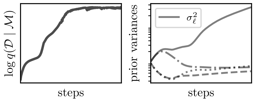
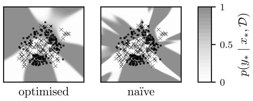
Figure 2:Using the Laplace-approximated marginal likelihood for online model selection of the prior variances on a small Bayesian neural network on a 2D classification task. We see that the marginal likelihood converges to a local optimum over the course of training and that the optimised model is better regularised than a naïvely trained (overfitting) model. Adapted from Immer et al., 2021
Simple example
As a simple illustrative example of online model selection with the marginal likelihood, we will consider a small fully-connected neural network for a synthetic 2D classification task. We place a Gaussian prior over the weights and we assume that the prior variance is shared within each layer. That is, the th weight in the th layer will have the prior . Our hyperparameters to select are now these layerwise variances, so .
We see in Figure 2 that our estimate of the marginal likelihood increases monotonically over the course of training and seems to converge to a local optimum. We also see that the prior variances indeed change during training and also seem to converge. The final model achieves a lower training accuracy compared to a naïvely trained model, but a higher test accuracy. This indicates that our selected model is better regularised and overfits less, in line with the Occam’s razor effect of the marginal likelihood. The visual smoothness of its decision boundary supports this conclusion.
On the risk of overfitting
Based on the previous example and our arguments above, you may now be convinced that the Laplace marginal likelihood will always select the best model for you, no matter the circumstances. Unfortunately, you would be wrong about that. We do not want to hide the caveat that maximum marginal likelihood (ML-II)—much like standard maximum likelihood (ML-I)—carries the inherent risk of overfitting. In our previous examples, such as choosing between two model architectures or optimising layerwise prior variances, this has not been apparent because the number of models compared (or number of hyperparameters optimised) was small compared to both the number of parameters of the model and the number of datapoints. However, if we were to optimise a number of hyperparameters (or compare a number of models) larger than and , we may well overfit the model to the data.
In such cases, just like in standard maximum likelihood, one remedy is to make the hyperprior in Equation (2) more informative and thus regularise the optimisation. We could, for instance, have a separate prior for each weight that we optimise with the marginal likelihood, but then have strong hyperpriors and that regularise these two parameters to some reasonable values unless the marginal likelihood really provides strong evidence for different ones. For a more in-depth discussion on the risks of overfitting with the marginal likelihood in model selection and the use of hyperpriors, see Ober et al. (2021).
Another remedy, proposed by Lotfi et al. (2022), is to compute the marginal likelihood not on the whole dataset, but only on a subset, similar to cross-validation. The authors call this the conditional log marginal likelihood (CLML). While this can in practice indeed reduce the overfitting effects, it inherits a lot of the computational challenges of standard cross-validation, most importantly the need to choose a validation split or to perform the procedure several times across different splits.
Connection to flat minima
A lot of the arguments we made above in Section Marginal likelihood for model selection hold for the true marginal likelihood . Based on some of the arguments in Chapter Introduction to Laplace approximations, you might wonder whether our approximation is not too crude for model selection purposes. If the true BNN posterior has exponentially many modes, each of which has potentially a non-Gaussian geometry, should we really believe that approximating the marginal likelihood with a single Gaussian on one mode is enough to judge the quality of the model? Indeed, the proof of the metaphorical pudding is in the eating, and we will see in the following section that the Laplace marginal likelihood can effectively be used for many model-selection use cases in practice. However, before we get to the empirics, there is one more conceptual argument we can offer to hopefully appease the sceptical reader.
If we have another look at our Laplace marginal likelihood criterion in Equation (11), we see that it has three parts: the prior, the likelihood, and the log determinant of the Hessian. That means that models will achieve a large marginal likelihood estimate if they are probable under the prior, fit the data well (in terms of the likelihood), and have a small determinant of the Hessian. The latter of these is clearly the most cryptic. What does a small determinant mean? Recall that we assume that we are at a local optimum, or have at least linearised our network or added a sufficiently strong prior, such that the Hessian is positive definite. That means that all its eigenvalues are positive. Since the determinant is the product of the eigenvalues, a small determinant means that the eigenvalues of the Hessian are small, which in turn means that the loss function (our negative log posterior) has low curvature in the region around —it is relatively flat.
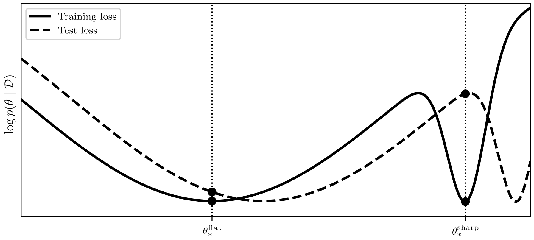
Figure 3:Here we show a loss landscape with a flat and a narrow minimum. As the loss landscape shifts from to , the solution still achieves a good performance, whereas the solution does not.
The idea that such flat minima can lead to better generalisation has been around for a while Hochreiter & Schmidhuber, 1997. In fact, it is quite intuitive, since it essentially means that small changes in do not lead to large changes in the loss, so even if we are a bit off from the true optimum and even if the loss landscape shifts a bit due to distribution shift in the test data, we will probably still achieve a relatively low test error. This intuition is also sketched in Figure 3. If this combination of train error (likelihood) and complexity measure (flatness) sounds like a PAC-Bayes bound to you, you are on the right track: flat minima have indeed been connected to PAC-Bayesian results Haddouche et al., 2025. Moreover, the deep learning community has embraced flatness-encouraging training criteria—similar to our marginal likelihood—for its purposes, such as the famous sharpness-aware minimisation SAM, Foret et al., 2021 or its Bayesian counterpart bSAM, Möllenhoff & Khan, 2023.
Use cases
As we have seen above, the Laplace marginal likelihood can be effectively used to select differentiable hyperparameters online, such as the prior variances or the likelihood noise, and to compare non-differentiable design choices post hoc, such as neural network architectures. These capabilities have been discovered by Immer et al. (2021) for modern deep learning models, and they have shown that this type of model selection is often cheaper and more effective than cross-validation. However, this type of hyperparameter tuning is by far not the only way the marginal likelihood can be used for model selection in deep learning. In recent years, different use cases have been developed, some of which have the potential to unlock entirely new application areas. While we cannot possibly provide a comprehensive overview of all of them, we will introduce a selection of the most interesting and creative ones in this section.
Feature selection
A common use case for model selection in Gaussian process models is feature selection via the automatic relevance determination (ARD) kernel Welch et al., 1992Rasmussen & Williams, 2006 (see also Chapter Introduction to kernel methods). This is a kernel in which each feature dimension has its own associated kernel length scale. These length scales can then be tuned using the marginal likelihood. One can perform a similar kind of feature selection in BNNs with the Laplace approximation, by performing model selection on the input weights. This is naturally more reasonable for data where the different input features have distinct semantic meaning, such as tabular data, than where they do not, such as images. One can even extend this idea to neural additive models (NAMs) Agarwal et al., 2021—that is, models where each input feature is passed to a separate neural network module—by performing model selection on the entire modules. Bouchiat et al. (2024) have shown that the Laplace marginal likelihood provides an effective way to select features in Bayesian NAMs and even further improve their interpretability through its Occam’s razor effect.
Neural network pruning
The aforementioned feature selection, in its simplest implementation, amounts to removing weights from the input layer. This suggests the idea that one might also be able to remove weights from deeper layers. Indeed, this is the basic premise of the research field of neural network pruning Cheng et al., 2024. There are two major approaches to pruning: unstructured pruning, where weights across the whole weight matrix are removed, and structured pruning, where entire rows or columns of the weight matrix are removed (this corresponds to removing neurons from the layer). Note that while the latter approach is more aggressive, it is the only one that immediately leads to computational gains, since the former approach just makes the matrix more sparse, but not smaller. Dhahri et al. (2024) have shown that the Laplace marginal likelihood can be used to improve pruning in both settings, through its Occam’s razor effect, which encourages the neural networks to only use just as many weights as are needed for a given task. They have also shown that the Laplace posterior offers a simple yet effective pruning criterion: the log posterior density evaluated at 0.
Invariance learning
While the previous two use cases are still intuitively connected to our original model selection examples, as well as to existing applications in other models such as Gaussian processes, Immer et al. (2022) propose to use the marginal likelihood for a more creative task: learning invariances from data. While invariances are commonplace in the context of designing invariant neural network architectures by hand (e.g., convolutional neural networks), there are many applications where invariances may be present in the data but the user does not know them. Following the approach from Wilk et al. (2018), Immer et al. (2022) suggest using the following parameterisation of a generic invariant function:
Here, is the neural network, is the desired invariant function, is a data augmentation distribution, with respect to which the function should be invariant, and are hyperparameters controlling this augmentation distribution. The Laplace marginal likelihood can now be used to select online during training and therefore enables learning a function that discovers the invariances directly from the data within a single training run. Immer et al. (2022) show that this can faithfully recover known invariances and can drastically improve data efficiency on real datasets.
Probing
In addition to the bona fide model selection use cases introduced above, finally, the marginal likelihood can even be used for applications that—on the surface—do not look like model selection, such as probing. Probing is a common interpretability tool in language models, and it tries to answer the question of whether the latent representations of these models encode certain properties of their inputs. For instance, people might wonder “Does BERT encode the concept of verb tense?”. To answer this, there is a long line of work trying to take these latent encodings and fitting different simple readout functions to them, such as linear functions, to predict the property of interest, in this case, verb tense Belinkov, 2022. But what if the encodings do not encode the property linearly but quadratically? Then the linear probe might not perform well, but arguably, the property is still encoded. However, a quadratic model is more complex than a linear one, so maybe one should count this property as less well encoded than in a set of encodings where a linear probe would suffice. That again sounds suspiciously like Occam’s razor, and indeed Immer et al. (2022) have shown that one can treat the problem of jointly selecting encodings and probes to predict the desired property as a model selection problem and use the Laplace marginal likelihood for a fair apples-to-apples comparison between different models. This shows that the tools presented in this chapter are much more widely applicable than one might naïvely expect, when one is a bit more creative in the interpretation of what model selection might look like.
- Sober, E. (2015). Ockham’s Razors: A User’s Manual. Cambridge University Press.
- MacKay, D. J. (2003). Information theory, inference and learning algorithms. Cambridge university press.
- Mackay, D. J. C. (1992). Bayesian methods for adaptive models [Phdthesis]. California Institute of Technology.
- Rasmussen, C., & Ghahramani, Z. (2000). Occam’s Razor. In T. Leen, T. Dietterich, & V. Tresp (Eds.), Advances in Neural Information Processing Systems (Vol. 13). MIT Press.
- Fong, E., & Holmes, C. C. (2020). On the marginal likelihood and cross-validation. Biometrika, 107(2), 489–496.
- Shawe-Taylor, J., & Williamson, R. C. (1997). A PAC analysis of a Bayesian estimator. Proceedings of the Conference on Learning Theory (COLT).
- McAllester, D. A. (1998). Some PAC-Bayesian theorems. Proceedings of the Eleventh Annual Conference on Computational Learning Theory, 230–234.
- Alquier, P. (2024). User-friendly Introduction to PAC-Bayes Bounds. Foundations and Trends in Machine Learning, 17(2), 174–303.
- Pérez-Ortiz, M., Rivasplata, O., Shawe-Taylor, J., & Szepesvári, C. (2021). Tighter Risk Certificates for Neural Networks. Journal of Machine Learning Research, 22(227), 1–40.
- Germain, P., Bach, F., Lacoste, A., & Lacoste-Julien, S. (2016). PAC-Bayesian Theory Meets Bayesian Inference. In D. Lee, M. Sugiyama, U. Luxburg, I. Guyon, & R. Garnett (Eds.), Advances in Neural Information Processing Systems (Vol. 29). Curran Associates, Inc.
- Neyman, J., & Pearson, E. S. (1933). IX. On the problem of the most efficient tests of statistical hypotheses. Philosophical Transactions of the Royal Society of London, Series A: Containing Papers of a Mathematical or Physical Character, 231(694–706), 289–337.
- Immer, A., Bauer, M., Fortuin, V., Rätsch, G., & Emtiyaz, K. M. (2021). Scalable Marginal Likelihood Estimation for Model Selection in Deep Learning. In M. Meila & T. Zhang (Eds.), Proceedings of the 38th International Conference on Machine Learning (Vol. 139, pp. 4563–4573). PMLR.
- Lin, J. A., Antoran, J., & Hernández-Lobato, J. M. (2023). Online Laplace Model Selection Revisited. Symposium on Advances in Approximate Bayesian Inference (AABI), 5.
- Ober, S. W., Rasmussen, C. E., & van der Wilk, M. (2021). The promises and pitfalls of deep kernel learning. In C. de Campos & M. H. Maathuis (Eds.), Proceedings of the Thirty-Seventh Conference on Uncertainty in Artificial Intelligence (Vol. 161, pp. 1206–1216). PMLR.
- Lotfi, S., Izmailov, P., Benton, G., Goldblum, M., & Wilson, A. G. (2022). Bayesian Model Selection, the Marginal Likelihood, and Generalization. In K. Chaudhuri, S. Jegelka, L. Song, C. Szepesvari, G. Niu, & S. Sabato (Eds.), Proceedings of the 39th International Conference on Machine Learning (Vol. 162, pp. 14223–14247). PMLR.