Linearised Laplace approximations
The previous chapter showed a computationally lightweight Gaussian approximation to the true posterior on the parameter space . Our final goal is to use this Gaussian measure to make decisions based on the model’s output: its predictions feed into the risks and utilities that downstream tasks optimise (Chapter Analytic, low-cost functionality from Laplace). To this end, we first quantify the predictive uncertainty of our network on the output space by turning it into a Gaussian process (GP). Figure 1 previews the pipeline, from the maximum a posteriori (MAP) estimate to the predictive distribution.
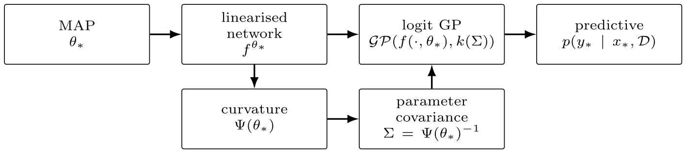
Figure 1:The linearised Laplace pipeline. The linearised network and parameter covariance jointly determine the logit Gaussian process, which induces a predictive distribution.
Linearisation
To turn an arbitrary (differentiable) neural network parameterised by into a Gaussian process, we use two ingredients: linearisation in the parameter space and the previously introduced Laplace approximation.
We first introduce the concept of the linearised network as the first-order Taylor approximation of network around parameters :
where is the network Jacobian evaluated at .[1] Analogously to Equation (1), we define the regularised empirical risk of the linearised network with parameters as
Unless explicitly stated otherwise (e.g., in the prior-only discussion in Section The Prior), we fix the linearisation point at a minimiser of the original regularised empirical risk :
that is, we set . Linearisation itself only requires differentiability of at . The Laplace approximation needs more: must be a local minimiser of with zero gradient, and the resulting precision must be positive definite after adding the prior curvature. We note that shares its value and its parameter Jacobian with at , so and is a stationary point of , too. Because is affine in , convexity of in makes each loss term convex in ; with a strictly convex , the risk is then strictly convex in , hence is its unique minimiser.
Following Section Laplace approximations are local and differential, the Laplace approximation using the regularised empirical risk of the linearised network yields the parameter-space Gaussian measure with
The curvature of the linearised network’s regularised empirical risk differs from the Hessian in Equation (7) for networks that are not piecewise affine in their parameters (except at the non-generic parameter values where all training residuals vanish). The difference is that , as defined in Equation (4), discards the network’s parameter curvature (and higher-order derivatives) and only retains the curvature of the loss function over the model outputs. The advantages of this modelling choice are summarised in Section Advantages of Using the Linearised Network.
An important property of Gaussian measures is their closure under affine transformations, stated formally below.
As such, the linearised network pushes the parameter posterior forward, via the affine map of Equation (1), to a Gaussian in the output space (the logit space in classification). In the network-output variable (the logits, which the loss takes as its first argument), this measure is
This result already equips the network with a probability measure in its output space (or logit space in classification) for every input . A Gaussian process is an even more powerful construction, capable of modelling a Gaussian measure over any finite set of inputs, not just a single one. The linearised network equipped with its parameter-space Laplace approximation defines a Gaussian process with the following (Mercer) kernel:
Advantages of Using the Linearised Network
We perform the Laplace approximation w.r.t. (with ) instead of the regularised empirical risk of for multiple reasons.
First, the Hessian of the regularised empirical risk of (Equation (7)) is not guaranteed to be positive definite, preventing us from interpreting it as the inverse covariance matrix of our approximate Gaussian posterior over the parameters .[2] In second-order optimisation, the lack of positive definiteness also prohibits using the inverse Hessian as a preconditioner. However, the Hessian of the regularised empirical risk of , with a strongly convex regulariser, is guaranteed to be positive definite.
Second, the Hessian of the regularised empirical risk of is considerably cheaper to use than that of , allowing Laplace approximations to scale to deep learning architectures (see Section The Fisher).
There are thus two uses of the linearised model. First, it defines the curvature and hence the parameter-space Gaussian posterior approximation. Second, it defines the predictive pushforward in Equation (13). Earlier work on Laplace approximations for neural networks MacKay, 1992Ritter et al., 2018 sampled parameter configurations from the parameter-space Gaussian and calculated predictive quantities from the nonlinear predictions . This loses the exact output-space Gaussian distribution available from linearisation and yields no posterior GP. Lawrence (2000) shows empirically that this approach is prone to underfitting: the predictive becomes too uncertain even on in-distribution data points. Immer et al. (2021) identify the core reason for performance loss as a mismatch between the model in which we perform approximate Bayesian inference (the linearised network ) and the model we use for prediction (the nonlinear network ). Figure 2 visualises this underfitting and the low-density samples drawn under the true posterior. See also Immer et al. (2021, Fig. 3). By using the linearised network to make predictions and not only to calculate the curvature, the approximation remains internally consistent.
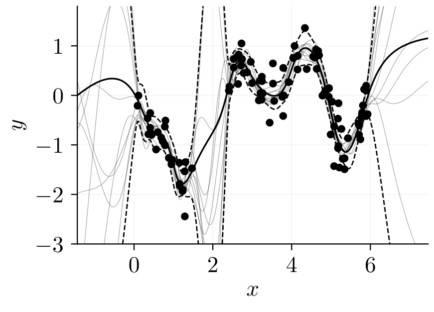
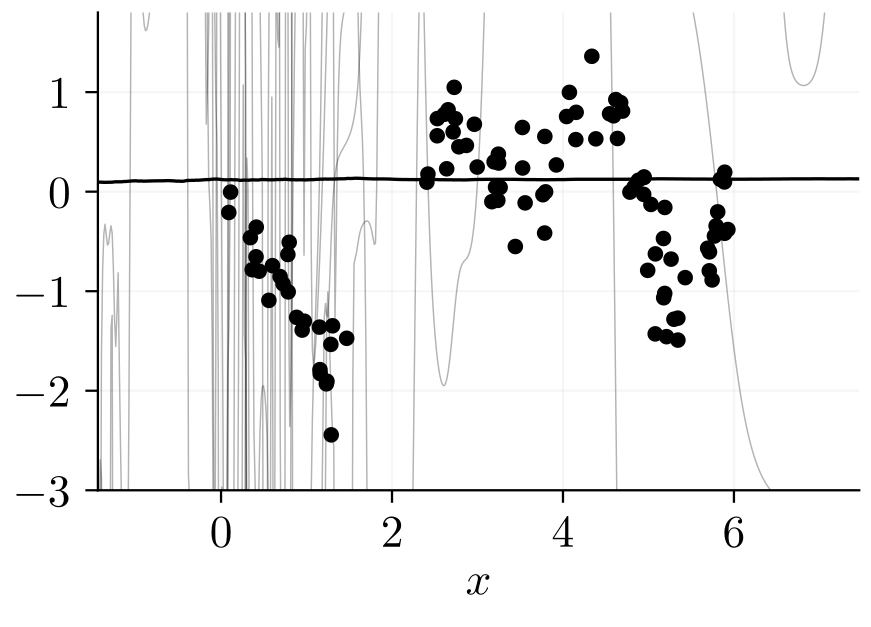
Figure 2:The same full Laplace posterior under two predictive rules on a one-dimensional regression example from the code accompanying Immer et al. (2021). Both panels use the same parameter-space approximate posterior and the same ten parameter draws. They differ only in how each parameter draw becomes a function-space sample called a sample path in the GP literature. Panel (a) sends each draw through the linearised network , the model consistent with the parameter-space Laplace approximation. Panel (b) sends the draws through the original nonlinear network . Solid curves are predictive means; dashed curves show pointwise credible intervals. The linearised Laplace approximation in Panel (a) yields a GP; therefore, the output-space quantities are available in closed form. The (nonlinear) Laplace approximation in Panel (b) yields an intractable output mean and covariance, which we approximate with two million Monte Carlo samples. The nonlinear scheme is far more uncertain over the training inputs and its mean severely underfits. The linearised Laplace approximation yields consistent function-space uncertainty.
The Prior
The Gaussian process determined by the posterior parameter-space covariance matrix is tied to the dataset , as is the Hessian of the linearised model’s regularised empirical risk over . It is worth spending some time on the case when the neural network has not been exposed to any dataset yet. In this case, the model’s behaviour is determined by its architecture and by the prior over the parameters.
For a non-Gaussian parameter prior , a Laplace approximation to the prior is centred at a local maximum of , analogously to Equation (6). Its precision is the negative log-prior Hessian,
For the construction that follows, we specialise to a Gaussian prior centred at the linearisation point,
where can be any chosen initialisation. The prior’s mode is , so the linearisation and the Laplace approximation of the prior share the same centre, and the precision above evaluates to . Pushing this prior through the linearised network gives the kernel ,
The kernel comes from the same pushforward as the posterior GP kernel in Equation (14). Compared with it, the data-dependent pair is replaced by the dataset-independent pair . This kernel is known as the Neural Tangent Kernel (NTK) Jacot et al., 2018.[3] It differs from the neural network Gaussian process (NNGP) kernel: the NNGP kernel is the covariance of random network outputs and under a random initialisation distribution, while the NTK is the covariance of the linearised network outputs and under the prior . As the network width is taken to infinity in a specific way, both kernels are convergent. Where these limits exist, they are different deterministic kernels.
The NTK determines the function-space trajectory of during full-batch gradient flow training on the average empirical loss via the Ordinary Differential Equation (ODE)
where is the time variable of the gradient flow and is the NTK of . Jacot et al. (2018) show that in the infinite-width limit of fully-connected neural networks with the so-called NTK initialisation, the NTK stays constant during training, and the convergence of optimisation is related to the positive definiteness of the NTK. However, the NTK of regular, finite-width neural networks is not constant and must be recomputed at every evaluation point.
From a modelling perspective, putting an isotropic Gaussian prior over the parameters is seldom well-motivated. However, the framework of Laplace approximations is compatible with interpretable function-space priors. Cinquin et al. (2024) define Laplace priors using a prior Gaussian process. In particular, the negative log-prior is, up to an additive constant, equal to the squared Reproducing Kernel Hilbert Space (RKHS) norm of the difference between the linearised network and the mean of the prior Gaussian process . This negative log-prior is also used as a regulariser during training. As specifying the Gaussian prior in the function space only requires knowledge about the function’s behaviour and not about the parameter space’s structure, the framework of Cinquin et al. (2024) allows domain experts to directly encode functional behaviour in the Bayesian inference problem.
The Fisher
In Section Linearisation, we glossed over the curvature matrix defined in Equation (4). This matrix and its components give an information-geometric interpretation to Laplace approximations, warranting its own chapter (Chapter The differential geometric perspective on Laplace).
Consider the regularised empirical risk of the linearised network (Equations (1) and (2)). Under the assumption of Equation (2) applied to the linearised network, the term
is equal, up to an additive constant, to the negative log-likelihood of the dataset under the model, , whereas the term equals the negative log-prior, , again up to an additive constant.
Writing out the Hessian of evaluated at , we obtain
called the Generalised Gauss-Newton matrix (GGN). In this section, we show that this matrix is equivalent to the Fisher Information Matrix for a family of loss functions, which is a natural (usually degenerate) Riemannian metric for statistical manifolds parameterised by the model (Section The Fisher Metric).
Consider the statistical manifold
with conditional independence structure , whose in-depth study we defer to Chapter The differential geometric perspective on Laplace. The distribution represents the likelihood parameterised by a neural network and is the ground-truth input distribution. A natural notion of separation between probability distributions on this manifold is the Kullback-Leibler (KL) divergence:
The KL divergence is not a valid metric, as it is non-symmetric. However, for parameters and and , the KL divergence’s second-order Taylor approximation around is given by
Both the zeroth- and first-order terms vanish (the former because , the latter because the expected score is zero, Equation (27)), leaving the quadratic Fisher term as the leading contribution. At each parameter , the bilinear form on tangent vectors is a valid Riemannian metric over manifold (up to the identifiability of parameters; see Chapter The differential geometric perspective on Laplace). The matrix
is called the Fisher Information Matrix (FIM) of the random variable distributed according to .
Differentiating the normalisation under the integral sign and using gives the zero-mean score,
Differentiating once more yields the two equivalent forms of the Fisher information,
The FIM of independent random variables is additive. In particular, for i.i.d. random variables , the FIM is times that of a single random variable :
In the following, we use the notation for the FIM of a single random variable distributed according to .
Using Equation (25), the utility of the FIM becomes clear in second-order optimisation. In particular, consider the objective
for some constant . The intuition behind this objective is that we want to minimise our model’s non-regularised empirical risk while limiting how much the likelihood induced by the model changes, irrespective of the curvature of the loss surface. To find an approximate minimiser of the objective in Equation (30), we consider the quadratic approximation to our constraint in Equation (25) and linearise the empirical risk around the current parameter :
Substituting in the linearised empirical risk and quadratic constraint, our objective becomes
The above is a convex quadratically constrained linear program. When is positive definite and , the optimum lies on the boundary of the constraint ellipsoid and can be found in closed form with Lagrange’s method, yielding
In particular, the optimal update direction is given by the so-called natural gradient with a magnitude that is a function of the constant . Natural-gradient methods are developed in detail in Chapter Natural-gradient-based variational inference.
In practice, we replace the unknown distribution of inputs with the empirical distribution w.r.t. training set :
The corresponding FIM approximation becomes
Using the chain rule w.r.t. the model’s output , we obtain
Here the network’s own second-order term vanishes under the expectation by the zero-mean score in (Equation (27) applied to ), which is why the linearised and nonlinear networks share the same . The expectation over model outputs for each input can be expensive to compute. One approach to mitigate the cost is the Monte Carlo approximation:
with . For small , we obtain a rather crude but cheap approximation. An alternative approach is to first rewrite as
(Equation (28), applied to ), then substitute the ground-truth labels instead of approximating the expectation:
called the Empirical Fisher Information Matrix (EFIM). While this substitution may seem natural, Kunstner et al. (2019) show that it has a detrimental effect for optimisation, where the predicted and ground-truth labels can be significantly different, especially at the beginning of training. However, for the Laplace approximation, we use a MAP estimate, which, if it generalises well, approximates the ground-truth label distribution well.
For a wide family of likelihoods, one does not have to approximate the Fisher by Monte Carlo. This allows us to connect the FIM to the GGN under some assumptions. Identifying and using Equation (1), in the case when the Hessian of the negative log-likelihood loss does not depend on the target , the GGN is equal to the FIM (up to a constant scaling factor):
In fact, the difference in the scaling factor has a natural interpretation. Previously, we saw that is the FIM of the random variable distributed according to and that the FIM is additive for independent random variables. Therefore, under this assumption, the GGN is equal to the FIM w.r.t. i.i.d. observations distributed as (and not as ).
The requirement of the loss Hessian not depending on the target might seem arbitrary. However, this property is satisfied by a wide family of likelihoods, called exponential families.
First, we state some facts about simple parameterisations.
Parameterisations via neural networks are more delicate. The following proposition gives a necessary and sufficient condition for Equation (40).
The above statement on neural network parameterisations covers the most popular loss functions in classification and regression. In classification, the cross-entropy loss is the negative log-likelihood of a categorical distribution parameterised by our neural network. The logits are the categorical’s natural parameters, so with the identity link the cross-entropy loss satisfies Proposition 3 in its affine special case. Similarly, the loss for regression satisfies Proposition 3 with .
A word of caution is in order: the GGN/FIM alone is usually degenerate; thus, it does not serve as a valid precision matrix for the Laplace approximation. Considering a single input-label pair , the term
is a positive semidefinite (PSD) matrix, as the loss Hessian is positive semidefinite. For softmax cross-entropy, this Hessian is , which is rank deficient as the softmax is shift-invariant. Usually, the GGN, that is, the sum of these matrices over the training dataset, is still rank deficient. However, adding the Hessian of the strongly convex regulariser term to the GGN results in the positive definite matrix
which is the Hessian of the regularised empirical risk of the linearised model, . This justifies using this matrix as a parameter-space precision in the Laplace approximation (Equation (6)).
With the curvature in hand, we can place the NTK of Section The Prior and the posterior GP kernel of Equation (14) in a single frame. Both are Jacobian Gram matrices in a parameter-space metric ; they differ in the expansion point ( for the NTK, for the posterior kernel) and in the metric . Preconditioning the gradient flow of Equation (19) by multiplies the parameter velocity by , inserting between the Jacobians and replacing its kernel with , holding the expansion point fixed and changing only the metric. Vanilla gradient descent uses the Euclidean metric and recovers the NTK, the isotropic-prior pushforward. Regularised natural-gradient descent Amari, 1998 uses , the GGN/Fisher curvature plus the prior precision (Equation (43)) at the current parameters. We call the resulting kernel the natural-gradient NTK. Because is positive definite at every , the natural-gradient NTK governs the dynamics all along training, even where the gradient is nonzero and no Laplace posterior exists. It coincides with the posterior GP kernel Immer et al., 2021 only at a posterior mode , as the Laplace approximation requires. The parameter-space metric thus determines both the predictive uncertainty, through the Gaussian we push forward, and the optimisation geometry, through the descent the function follows.
Scalable Curvature Approximations
The GGN of the linearised network (cf. Equation (22))
is dense in general and far too large to form for modern neural networks. We therefore seek structured surrogates that (i) are cheap to store and invert, yet (ii) retain meaningful parameter correlations. Table 1 compares the three curvature proxies we develop: the diagonal, low-rank, and Kronecker-Factored Approximate Curvature (KFAC) approximations. Scalable variants of these curvature approximations are developed further in Chapter Scalable Laplace approximations, and last-layer inference is treated in Chapter Last-layer inference.
A simple baseline is the diagonal , which is trivial to store and invert, though calculating it efficiently requires care. However, it encodes an independence assumption between all parameters, destroying the often-crucial within-layer correlations carried by . This tends to hurt the utility of the downstream uncertainty estimates Daxberger et al., 2021.
Table 1:Common scalable curvature approximations for linearised Laplace. Here and are the input and pre-activation dimensions of layer .
| Approx. | Storage | Cov.-vec. | Inversion | Correlations | Blind spot |
|---|---|---|---|---|---|
| Diag. | Elementwise division | Elementwise | None across parameters | Misses coupled directions | |
| Low-rank | Products with | Woodbury | Top eigenspace of | Misses broad low-curvature directions | |
| KFAC | Kronecker identities | Factor eigensystems | Within-layer Kronecker | Drops cross-layer couplings |
Low-rank GGN Approximations
A scalable yet expressive alternative is a low-rank approximation of . As is symmetric for any , it possesses an eigendecomposition with real eigenvalues of the form
where is an orthogonal matrix (i.e., a matrix with orthonormal columns/rows) and is a diagonal matrix.
For , the th column of , and , the th diagonal entry of , it holds that . We follow the convention . In the following, we drop the dependence of and its factors on for brevity.
We now seek a good low-rank approximation to , as this reduces the sizes of the objects we need to handle. Since , its eigenvalues are nonnegative, so the algebraically largest coincide with the largest in magnitude. The Eckart–Young–Mirsky theorem Eckart & Young, 1936 states that the objective
is minimised by where is the first columns of and holds the first eigenvalues of . This result holds for both the spectral norm and the Frobenius norm . Therefore, one obtains an optimal low-rank approximation to in the above sense by computing the first eigenvalues and eigenvectors of . Storing this low-rank approximation requires storing values instead of .
The most naive way to compute is first calculating the eigendecomposition and then truncating it to the first eigenpairs. However, this strategy does not resolve the infeasibility of storing the full eigendecomposition with values. Instead, one uses efficient matrix-free schemes such as the Locally Optimal Block Preconditioned Conjugate Gradient (LOBPCG) method Knyazev, 2001 or Lanczos iterations Lanczos, 1950 to obtain the low-rank decomposition. Notably, these algorithms only require matrix-vector products with the GGN to obtain the top eigenpairs, which does not require representing the entire matrix in memory.
The low-rank representation is particularly handy, as for simple priors, such as isotropic Gaussians, calculating the approximate covariance matrix is just as efficient as working with the low-rank GGN. Let be the Hessian of the negative log-prior , that is, the prior-curvature term of the precision (Equation (43)). Then the Woodbury matrix identity yields
In particular, for isotropic Gaussians, ,
In words: a diagonal-plus-low-rank matrix has a diagonal-plus-low-rank inverse. Multiplying by such a matrix is efficient and does not require forming a matrix. For a vector , we first calculate , then elementwise multiply by the diagonal entries in , then map the result back to with and add the diagonal term .
Kronecker-Factored Approximate Curvature
A complementary path towards scalable approximate curvature representations assumes independence between layers only, while retaining rich within-layer parameter correlations via a Kronecker factorisation. This idea underlies KFAC, which has recently seen wide use as a scalable curvature proxy Martens & Grosse, 2015. In this section, we give an introduction to KFAC for dense linear layers and refer to Dangel et al. (2025) for a more detailed and general exposition of KFAC.
Consider layer with weights , input activation , and pre-activation .[4] Let denote the network output. Let denote the Jacobian of w.r.t. , where flattens its input by stacking its columns. For datum , define the output-space curvature , so . Writing with , the corresponding layer block of the GGN can be expressed as
with , where is the Jacobian of the network output w.r.t. this layer’s pre-activation .[5] Thus, the sum over is over the network output curvature factor, while lives in the layer pre-activation space.
For a linear layer, the output-parameter Jacobian has the form where denotes the Kronecker product. Noting the Kronecker properties and for compatible matrices , we get
The KFAC approximation then pulls the Kronecker product outside the sum:
Thus, the layer block is approximated by
Stacking layers and neglecting inter-layer couplings yields a block-diagonal curvature with Kronecker blocks .
The Kronecker form is efficient to store. While the dense GGN for a single linear layer has entries, the Kronecker factorisation only requires storing and , that is, a total of values. The block-diagonal layer approximation then avoids storing cross-layer blocks. One can also calculate efficient covariance-vector products without forming a dense matrix by leveraging the cached eigendecompositions of the Kronecker factors and standard Kronecker identities. This property is more involved to show than in the case of low-rank approximations; refer to Dangel et al. (2025) for more details.
The Predictive
Equation (13) gives a Gaussian distribution in the output space for input . For regression, this distribution is called the predictive distribution: its mean encodes the average prediction under the parameter-space posterior and the linearised model, and its covariance structure quantifies the uncertainty in the prediction, including correlations of the outputs. Figure 3 shows a one-dimensional regression example of the linearised Laplace approximation.
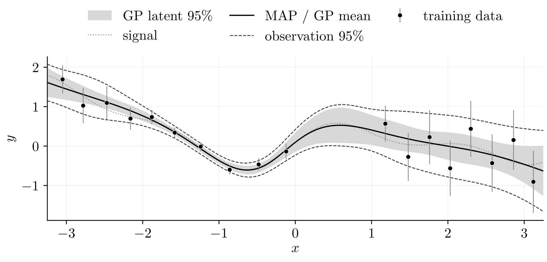
Figure 3:A one-dimensional regression example with irregular inputs and input-dependent observation noise. The model is a neural network with a Bayesian last layer, so the linearisation is exact and the linearised GP yields the exact posterior predictive. The shaded region shows the pointwise latent GP interval, while the dashed curves add the input-dependent observation variance.
In classification, however, we are interested in obtaining a second-order distribution (a distribution over distributions) over the categorical distributions of a discrete set of labels. To this end, one has to map the logit-space Gaussian measure in Equation (13) through an activation function onto the ()-dimensional probability simplex:
where is the mapping from an input to the logit-space Gaussian distribution given by the Laplace-approximated network, is the set of Gaussian measures on the logit space , is the set of probability measures on the simplex, and pushes forward the Gaussian probability measures through the activation function. The roman is the network with its parameter posterior pushed through it: the affine pushforward of the Laplace posterior along the linearised network, giving as in Equation (13). The italic plugs in the point estimate and returns a single logit vector; the roman returns the full logit-space Gaussian, whose mean is exactly that italic vector. All parameters in the support of the Laplace posterior are taken into account rather than a single one being held fixed, so takes only the input. In words, is the composition of the Laplace-approximated neural network outputting logit-space Gaussian distributions, , and the pushforward map through the activation function that gives us a distribution over probability vectors.
In most cases, this activation function is the softmax, defined as ,
In this case, there exists no closed-form expression for given input . Further, , called the posterior predictive, is also intractable. However, sampling from is efficient, as it only requires sampling from the logit-space Gaussian and pushing these logit samples forward through the activation function. Thus, in practice, one resorts to Monte Carlo integration, that is, drawing samples from and calculating their empirical average. Similarly, one can approximate other derived quantities, such as the expected entropy , through Monte Carlo sampling. Such derived quantities are often used in the field of uncertainty disentanglement, where different quantities capture different sources of uncertainty Mucsányi et al., 2024. These uncertainty estimates are applied to selective classification in Chapter Confidence-based selective classification.
The main issue with the above schemes is the requirement of sampling: the error of Monte Carlo integration decreases as the inverse square root of the number of samples , meaning that to reduce the error by three orders of magnitude, one needs a million samples. Standard softmax-cross-entropy integration cannot avoid this sampling cost without incurring significant approximation error. However, some output activation functions admit a closed-form posterior predictive. For a single output, integrating a normCDF (probit) link against a Gaussian is exact, and the logistic sigmoid admits a classical probit approximation MacKay, 1992. Mucsányi et al. (2025) show that the normalised elementwise sigmoid and normCDF functions yield closed-form predictives that have strong approximation guarantees and are naturally compatible with more performant training objectives than the standard softmax-cross-entropy objective. Further, derived quantities such as the expected entropy can also be obtained in closed form by matching the moments of the Gaussian pushforward distributions with Dirichlets. The change in the training objective comes at no cost: models trained this way become better calibrated while providing sample-free posterior predictives and other derived quantities. Therefore, Laplace approximations in classification can be formulated in a purely sample-free fashion, with theoretical guarantees. Figure 4 compares the MAP, Monte Carlo softmax, and sample-free probit predictives on a two-dimensional example, together with the predictive entropy.
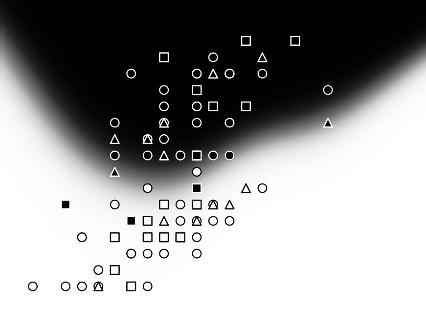
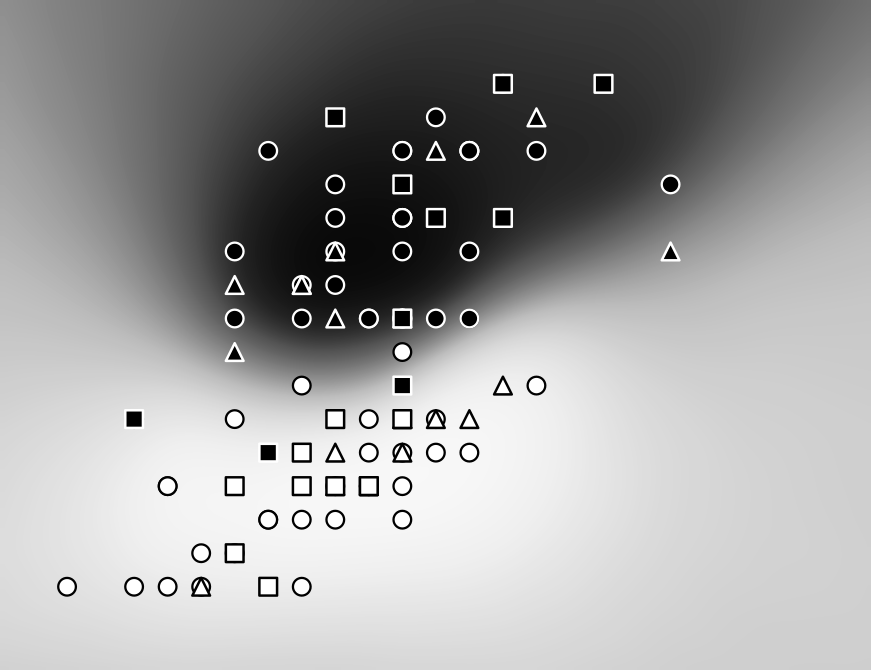
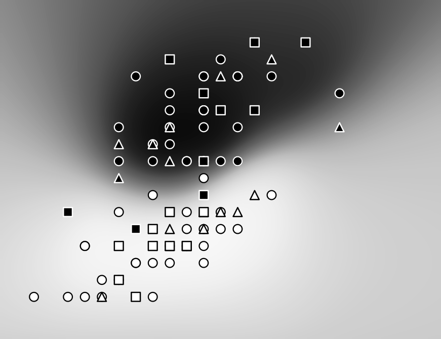
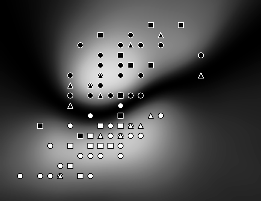
Figure 4:Two-dimensional binary classification with a Laplace approximation to the last layer of a fixed-feature network on the Iris dataset. The inputs are the measured sepal width and petal width. White denotes Iris versicolor and black denotes Iris virginica. Circles are training points, triangles are validation points, and squares are test points. The prior precision is selected on the validation set by log score. Panels (a)–(c) show the probability of the black class for the MAP predictor, the softmax posterior predictive estimated by Monte Carlo sampling, and the sample-free probit approximation. Panel (d) shows the predictive entropy computed from the Monte Carlo predictive. On the held-out test points, the MAP log score and Brier score are 0.433 and 0.122, while the Monte Carlo GP predictive gives 0.345 and 0.107, and the probit predictive gives 0.347 and 0.108—close to indistinguishable.
Note that this network is only linear in its parameters but is still nonlinear in its inputs .
For a finite-width network, this is sometimes called the empirical NTK at , and the NTK is reserved for networks in the infinite-width limit.
Bias terms are omitted for brevity.
For the squared loss, ; for cross-entropy, is the softmax Hessian.
- MacKay, D. J. C. (1992). A Practical Bayesian Framework for Backpropagation Networks. Neural Computation, 4(3), 448–472.
- Ritter, H., Botev, A., & Barber, D. (2018). A Scalable Laplace Approximation for Neural Networks. 6th International Conference on Learning Representations, ICLR 2018, Vancouver, BC, Canada, April 30 - May 3, 2018, Conference Track Proceedings.
- Lawrence, N. D. (2000). Variational Inference in Probabilistic Models [Ph.D. thesis]. Department of Computer Science.
- Immer, A., Korzepa, M., & Bauer, M. (2021). Improving predictions of Bayesian neural nets via local linearization. In A. Banerjee & K. Fukumizu (Eds.), Proceedings of The 24th International Conference on Artificial Intelligence and Statistics (Vol. 130, pp. 703–711). PMLR.
- Jacot, A., Gabriel, F., & Hongler, C. (2018). Neural Tangent Kernel: Convergence and Generalization in Neural Networks. In S. Bengio, H. Wallach, H. Larochelle, K. Grauman, N. Cesa-Bianchi, & R. Garnett (Eds.), Advances in Neural Information Processing Systems (Vol. 31). Curran Associates, Inc.
- Cinquin, T., Pförtner, M., Fortuin, V., Hennig, P., & Bamler, R. (2024). FSP-Laplace: Function-Space Priors for the Laplace Approximation in Bayesian Deep Learning. In A. Globerson, L. Mackey, D. Belgrave, A. Fan, U. Paquet, J. Tomczak, & C. Zhang (Eds.), Advances in Neural Information Processing Systems (Vol. 37, pp. 13897–13926). Curran Associates, Inc.
- Kunstner, F., Hennig, P., & Balles, L. (2019). Limitations of the empirical Fisher approximation for natural gradient descent. In H. Wallach, H. Larochelle, A. Beygelzimer, F. d’Alché Buc, E. Fox, & R. Garnett (Eds.), Advances in Neural Information Processing Systems (Vol. 32). Curran Associates, Inc.
- Amari, S. (1998). Natural Gradient Works Efficiently in Learning. Neural Computation, 10(2), 251–276.
- Daxberger, E., Kristiadi, A., Immer, A., Eschenhagen, R., Bauer, M., & Hennig, P. (2021). Laplace Redux - Effortless Bayesian Deep Learning. In M. Ranzato, A. Beygelzimer, Y. Dauphin, P. S. Liang, & J. W. Vaughan (Eds.), Advances in Neural Information Processing Systems (Vol. 34, pp. 20089–20103). Curran Associates, Inc.
- Eckart, C., & Young, G. (1936). The Approximation of One Matrix by Another of Lower Rank. Psychometrika, 1(3), 211–218.
- Knyazev, A. V. (2001). Toward the Optimal Preconditioned Eigensolver: Locally Optimal Block Preconditioned Conjugate Gradient Method. SIAM Journal on Scientific Computing, 23(2), 517–541.
- Lanczos, C. (1950). An iteration method for the solution of the eigenvalue problem of linear differential and integral operators. Journal of Research of the National Bureau of Standards, 45(4), 255–282.
- Martens, J., & Grosse, R. (2015). Optimizing Neural Networks with Kronecker-factored Approximate Curvature. In F. Bach & D. Blei (Eds.), Proceedings of the 32nd International Conference on Machine Learning (Vol. 37, pp. 2408–2417). PMLR.
- Dangel, F., Mucsányi, B., Weber, T., & Eschenhagen, R. (2025). Kronecker-factored Approximate Curvature (KFAC) From Scratch.
- Mucsányi, B., Kirchhof, M., & Oh, S. J. (2024). Benchmarking Uncertainty Disentanglement: Specialized Uncertainties for Specialized Tasks. In A. Globerson, L. Mackey, D. Belgrave, A. Fan, U. Paquet, J. Tomczak, & C. Zhang (Eds.), Advances in Neural Information Processing Systems (Vol. 37, pp. 50972–51038). Curran Associates, Inc.