Introduction to Laplace approximations - Handbook of Bayesian Deep Learning

Astute readers of the preceding chapter will have noticed that the methods introduced in Part 1 — Sampling methods come with a concerning amount of computational and memory overhead. Even a perfectly efficient Monte Carlo method, one that draws an i.i.d. sample from the posterior in every single step, still requires us to store multiple samples—entire copies of the parameter vector—in memory. At prediction time, we then have to compute the forward pass of the model for each of these samples. The number $k$ of samples enters at least multiplicatively into the computational cost $c$ of whatever it is we are doing with our neural network: We will pay a price of $\Omega(kc)$ (the Landau $\Omega$ . Yes, that’s a lower bound), both in memory and computation, to turn a non-Bayesian computation into a Bayesian one. At a time when prominent non-Bayesian deep models are already maxing out the capacity of the best multi-GPU workstations, this is a nonstarter, and arguably the main reason why Bayesian deep learning has acquired a reputation for unacceptably high computational cost.

This Part, however, will introduce a different, more practically minded way to endow neural networks with Bayesian uncertainty. Its history is just as old as that of sampling methods, and was born out of computational necessity in the early days of deep learning MacKay, 1992. In fact, it was originally invented in the early 19th century, long before digital computers Laplace, 1820, to turn intractable integrals into tractable ones, at any cost. As computation is once again a bottleneck in the deep learning age, Laplace approximations have re-emerged as a practical tool Khan et al., 2019Daxberger et al., 2021Immer et al., 2021 with new twists that push the envelope of automatic differentiation Dangel et al., 2020Dangel et al., 2025 and numerical linear algebra Cinquin et al., 2024. It also offers new perspectives on deep learning from the perspective of differential geometry Kristiadi et al., 2023Roy et al., 2024. As we will see, it now comes with great power, and grave dangers.

A linearized Laplace approximation on the most basic feed-forward perceptron f(x,\theta) = \theta_2 \cdot \operatorname{ReLU}(\theta_1 x + 1) for the dataset X=(1,-1),Y=(-1,-1), with regularizer \Omega(\theta)=0.2 \cdot \|\theta\|^2 and square loss. The grey contour lines denote the energy function. The black dot represents the minimum \theta_*; the thick black ellipses denote one (solid) and two (dashed) standard deviations of the Laplace approximation. The Gaussian approximation defined by the Laplace approximation clearly captures the local geometry, but not the full global shape of the posterior. 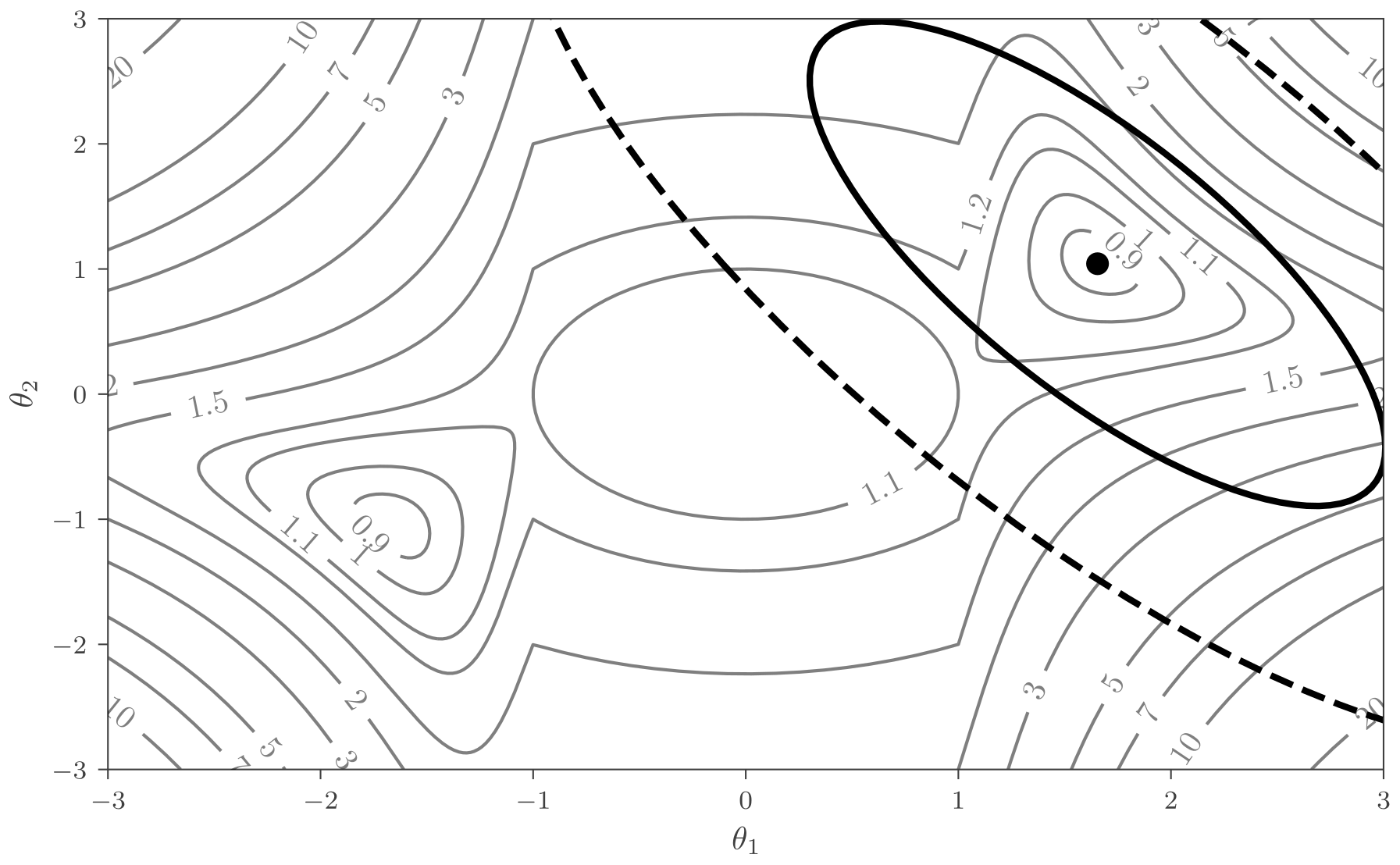— Figure 1:A linearized Laplace approximation on the most basic feed-forward perceptron $f(x,\theta) = \theta_2 \cdot \operatorname{ReLU}(\theta_1 x + 1)$ for the dataset $X=(1,-1),Y=(-1,-1)$ , with regularizer $\Omega(\theta)=0.2 \cdot \|\theta\|^2$ and square loss. The grey contour lines denote the energy function. The black dot represents the minimum $\theta_*$ ; the thick black ellipses denote one (solid) and two (dashed) standard deviations of the Laplace approximation. The Gaussian approximation defined by the Laplace approximation clearly captures the *local* geometry, but not the full *global* shape of the posterior.

Laplace approximations are local and differential¶

As in previous chapters, consider a differential program $f: \mathbb{R}^{D}\times\mathbb{R}^{P}\to\mathbb{R}^{C}$ mapping inputs $x\in\mathbb{R}^{D}$ to outputs $f(x,\theta)\in\mathbb{R}^{C}$ , parametrised by $\theta\in\mathbb{R}^{P}$ . Consider the regularized empirical risk $\regrisk\in\mathbb{R}$ defined as

\regrisk(\theta) = \sum_{n=1} ^N \ell(f(x_n,\theta),y_n) + \Omega(\theta).

(1)

with loss function $\ell\colon \mathbb{R}^{C} \times \mathbb{R}^{C} \to \mathbb{R}$ and regularizer $\Omega\colon \mathbb{R}^{P} \to \mathbb{R}$ , both strictly convex and twice continuously differentiable.^[1]

Also as in previous chapters, we interpret this function as an energy function, the unnormalised negative logarithm of a posterior:

\regrisk(\theta) = -\log p(Y \mid X, \theta) - \log p(\theta) + \text{const} = -\log p(\theta\mid \mathcal{D}) + \text{const}.

(2)

Definition 1

A Laplace approximation is any algorithm within a general class of methods that approximate $\regrisk(\theta)$ with a quadratic function

\regrisk(\theta) \approx \frac{1}{2}(\theta-\theta_*)^\top \Psi(\theta_*) (\theta-\theta_*) + \text{const},

(3)

where $\Psi(\theta_*)\in\mathbb{R}^{P\times P}$ is a second-order linear differential operator acting on $\regrisk(\theta_*)$ at the point $\theta_*\in\mathbb{R}^{P}$ . A Laplace approximation is thus defined by the tuple $(\theta_*,\Psi)$ , which we will call a point estimate and its curvature, respectively.

Under the assumption of Equation (2), any Laplace approximation is directly associated with an approximate Gaussian measure on the parameter space,

p(\theta\mid\mathcal{D}) =\frac{1}{Z(\mathcal{D})}\exp(-\regrisk(\theta))

(4)

p(\theta\mid\mathcal{D}) \approx \frac{1}{Z(\mathcal{D})}\exp\left(-\frac{1}{2}(\theta-\theta_*)^\top \Psi(\theta_*) (\theta-\theta_*)\right)

(5)

p(\theta\mid\mathcal{D}) = \mathcal{N}(\theta;\theta_*, \Psi^{-1}(\theta_*)).

(6)

The textbook, but impractical, version of the Laplace approximation arises from the Taylor expansion at a local minimizer of the regularized risk:

[\Psi(\theta)]_{ij} = \left[\nabla_\theta \nabla_\theta ^\top \regrisk(\theta)\right]_{ij} = \frac{\partial^2 \regrisk(\theta)}{\partial \theta_i \partial \theta_j}, \qquad \theta_* = \operatorname*{arg\,min}_{\theta\in\mathbb{R}^{P}} \regrisk(\theta).

(7)

That is, we pick a point $\theta_*$ where the gradient vanishes, and compute the Hessian there (the matrix $\Psi(\theta_*)$ being the matrix representation of the aforementioned operator, evaluated at $\theta_*$ ).

What is to like about Laplace?¶

Central to the appeal of Laplace approximations is that they are an analytic post-processing step that can be tagged onto the established way of training a deep model:

And that’s it! You now have a “Bayesian uncertainty” estimate in parameter space, in the form of the Gaussian from Equation (6). Let us spell out the advantages of this recipe, some more obvious, some less so, explicitly:

You get to keep your point-estimate. People who train neural networks, especially if it is a large model, spend extreme resources to find a good value $\theta_*$ . Even if this particular value may not hold up to the theoretical demands of Bayesian analysis, it nevertheless embodies a significant investment, so it is appealing to keep working with this valuable object. For Laplace, this point estimate turns directly into a posterior mean. And to state the obvious: The computation overhead of this part is strictly zero over whatever the training cost to begin with.
You get to use established tools. Constructing the Gaussian of Equation (6), requires precisely two computational tools: Automatic differentiation to get $\Psi$ , and numerical linear algebra, to find its (approximate) inverse. These are arguably the most powerful, reliable, optimised functionalities available to the machine learning engineer. They can be made extremely numerically robust and conveniently automated, or tailored for radical computational efficiency. And, using probabilistic numerical linear algebra, the discretisation and iteration error of these internal computations can be tracked for downstream consideration (More about numerical linear algebra tricks in Chapter Linearised Laplace approximations and Part 8 — Scalability).
Laplace is post hoc. Since $\Psi$ is only needed after $\theta_*$ has been found, its cost is not a function of the complexity of training. In fact, the construction of a Laplace approximation is effectively separated from training entirely, and can be done on a pre-trained model downloaded from the Internet. The only caveat is that, since $\Psi$ is a function of the regularized risk, we need access to the training data $\mathcal{D}$ – or some compressed representation thereof.
Laplace is analytical. Laplace approximations return a Gaussian probability measure, whose parameters are computed using optimization, automatic differentiation, and linear algebra. That is, a deterministic quantity – a probability density function – constructed deterministically. There is no source of randomness involved, apart from the potentially stochastic nature of training to find $\theta_*$ . As we will see in Chapter Analytic, low-cost functionality from Laplace, this makes Laplace approximations interesting for downstream applications and decisions that require analytic marginalization over the parameters.
Deep theoretical meaning. We will find in Chapters Linearised Laplace approximations and The differential geometric perspective on Laplace that the local differential nature of the curvature at the heart of Laplace approximations gives them profound theoretical connections, and intuitive interpretations. In fact, they open up a whole self-contained theory of deep learning founded on the differential geometry of the energy manifold associated with $\regrisk$ .
Laplace turns every deep network into a Gaussian process. In Chapter Linearised Laplace approximations, we will see that the Gaussian measure $\mathcal{N}(\theta;\theta_*, \Psi^{-1}(\theta_*))$ constructed by the Laplace approximation can be analytically pushed forward to the output space of the network $f(x,\theta)$ , where it manifests itself as a Gaussian process, whose mean-function is exactly the trained network $f(x,\theta_*)$ , and whose covariance function (kernel) is given by a structured object, a tangent kernel (developed further in Part 5 — Kernel methods). This is a powerful perspective for both practical and conceptual reasons: On the practical side, we can more or less directly transport a lot of notions from the Gaussian process literature to deep learning, recovering advanced functionality sorely missing from non-Bayesian deep learning. And on the conceptual side, the tangent kernel contains very specific terms that capture modular, interpretable statements about the role of the training data, the network architecture, and regularization that make deep learning more transparent and interpretable.

Practical Considerations¶

On first encountering Laplace approximations in deep learning, people tend to have one of two, mutually almost contradictory reactions:

Isn’t this too simplistic?¶

A Taylor-expansion? Really? From a fundamentalist Bayesian perspective, a quadratic function is a poor approximation of the posterior, with all its non-convex nonlinear glory (cf. Figure 1). But compared to the day-to-day practice of training deep networks, Laplace approximations are a big step forward, from a zeroth order approximation (a point estimate) to a second-order approximation (a Gaussian probability measure). They offer an easy gateway into the Bayesian world for the deep learning practitioner: Just take your trained model, compute a curvature, and Bob’s your uncle.

We should also be careful not to appeal to unrealistic ideals, but compare to realistic alternatives instead. The true posterior may be the theoretical target of all Bayesian analysis, but is completely intractable. All Bayesian methods that are actually accessible are approximations, of different nature. For example, if we draw an ensemble of $S\ll P$ samples $[\theta_s]_{s=1}^S$ from the posterior, and use it to construct a posterior covariance $\hat{\Psi}^{-1} = \frac{1}{S} \sum_{s=1}^S (\theta_s-\theta_*)(\theta_s-\theta_*)^\top$ over the parameters $\theta$ , that matrix $\hat{\Psi}$ will be of rank at most $S$ . If we use this object as a proxy for “posterior uncertainty”, we may severely over-estimate confidence intervals. A Laplace approximation might overlook nonlocal aspects of the posterior’s geometry, but it can construct an approximate covariance matrix of full rank.

Isn’t this too expensive?¶

Hang on, we need a Hessian over the parameter space? That’s a matrix of size $P\times P$ , so just storing it will create a memory overhead of $\mathcal{O}(P^2)$ . Oh, and then we need to compute its inverse!? That will incur a computational cost of $\mathcal{O}(P^3)$ , right? The flaw of such thoughts is that they use worst case statements about objects that are entirely under the user’s control.

It is better to think of the curvature $\Psi$ as a linear operator Dangel et al., 2025, a function mapping vectors to vectors. Such a function need not require the explicit instantiation of a matrix in memory. Chapters Linearised Laplace approximations and Analytic, low-cost functionality from Laplace will introduce several possible choices for this operator, spanning a range of computational and memory costs. These include the generalised Gauss-Newton approximation (Section The Fisher), Kronecker-factored approximate curvature, and diagonal approximations to the Hessian (Section Scalable Curvature Approximations). In fact, in Section Fixing overconfidence with calibrated uncertainty we will see that even the trivial choice $\Psi=\alpha I$ for an arbitrary $\alpha \in \mathbb{R}_+$ (i.e. just replacing the point estimate with an arbitrary Gaussian measure) already fixes some tangible, nontrivial pathologies of non-Bayesian deep learning.

Likewise, numerical linear algebra offers a rich toolbox of iterative, sparse, sketched, etc. methods to solve linear systems of equations of the form $\Psi x = b$ for $x$ without the need to even explicitly form an estimate of the matrix inverse $\Psi^{-1}$ (Section Low-rank GGN Approximations). And there are probabilistic versions of these methods that can partially track and estimate the error of their output e.g. Wenger et al., 2022Cockayne et al., 2019Wenger & Hennig, 2020. The memory and compute cost of Laplace approximations can thus be completely controlled by the user, opening up a wide spectrum of algorithms of varying quality and cost.

On the flip side, this also means that constructing Laplace approximations, just like training deep networks, is not a turnkey operation, and requires care and expertise. But emerging software tools increasingly encapsulate these choices, and provide abstraction layers that allow constructing Laplace approximations with a few lines of code.

All approximations are wrong¶

Despite all the arguments in their favour, Laplace approximations remain just that: approximations. Their local nature – the fact that they only use differential quantities evaluated at a single point in the parameter space – is both their principal strength and their principal weakness. As Figure 1 shows, the Gaussian posterior created by a Laplace approximation may not capture the geometry of the posterior – not even within the region of the parameter space delineated by one or two standard deviations of that Gaussian. And when intricate numerical routines are used to operate on the curvature operator $\Psi$ , their own errors can also severely erode the quality of the approximation.

Laplace approximations should thus best be viewed as an important tool of first resort. At least their most basic variants can be constructed on virtually any deep architecture, often with minimal overhead in both implementation and computation. They can be a powerful diagnostic tool, elucidating the interplay between data and architecture; and offer structured, controllable functionality for everyday requirements like uncertainty quantification, model adaptation, continual learning, and more. But whenever the stakes are high, for example in safety critical applications, or when uncertainty is used to draw scientific conclusions, additional safeguards are needed. In such settings, Laplace approximations may be paired with some of the other frameworks described in this book, to provide a more robust and calibrated uncertainty estimate.

Takeaways:

A Laplace approximation is a quadratic approximation to the log posterior associated with a deep model, interpreted as a Gaussian posterior on the parameter space, or a Gaussian process posterior on the predictive (logit) outputs of the model. Such approximations are constructed by first training a point estimate for the parameters in the “normal” way, then computing the curvature operator (or kernel) post hoc. By this nature, Laplace approximations are local and differential. On the one hand, this is a weakness, because they fail to capture global, non-linear structure in the posterior. On the other hand, this is a strength, because it allows the use of powerful automatic differentiation and matrix-free, probabilistic linear algebra, and provides theoretical descriptions of deep learning in the terms of differential geometry. The following chapters will provide further details on these aspects.

Footnotes¶

Note that convexity here is only assumed for the loss and regularizer. The full loss $\regrisk(\theta)$ is not generally convex, since the network $f$ is a nonlinear function of the parameters $\theta$ .
↩

References¶

MacKay, D. J. C. (1992). Bayesian Interpolation. Neural Computation, 4(3), 415–447.
Laplace, P. S. (1820). Théorie analytique des probabilités. Courcier.
Khan, M. E., Immer, A., Abedi, E., & Korzepa, M. (2019). Approximate Inference Turns Deep Networks into Gaussian Processes. In H. Wallach, H. Larochelle, A. Beygelzimer, F. d’Alché Buc, E. Fox, & R. Garnett (Eds.), Advances in Neural Information Processing Systems (Vol. 32). Curran Associates, Inc.
Daxberger, E., Kristiadi, A., Immer, A., Eschenhagen, R., Bauer, M., & Hennig, P. (2021). Laplace Redux - Effortless Bayesian Deep Learning. In M. Ranzato, A. Beygelzimer, Y. Dauphin, P. S. Liang, & J. W. Vaughan (Eds.), Advances in Neural Information Processing Systems (Vol. 34, pp. 20089–20103). Curran Associates, Inc.
Immer, A., Bauer, M., Fortuin, V., Rätsch, G., & Emtiyaz, K. M. (2021). Scalable Marginal Likelihood Estimation for Model Selection in Deep Learning. In M. Meila & T. Zhang (Eds.), Proceedings of the 38th International Conference on Machine Learning (Vol. 139, pp. 4563–4573). PMLR.
Dangel, F., Kunstner, F., & Hennig, P. (2020). BackPACK: Packing more into Backprop. 8th International Conference on Learning Representations, ICLR 2020, Addis Ababa, Ethiopia, April 26-30, 2020.
Dangel, F., Eschenhagen, R., Ormaniec, W., Fernandez, A., Tatzel, L., & Kristiadi, A. (2025). Position: Curvature Matrices Should Be Democratized via Linear Operators.
Cinquin, T., Pförtner, M., Fortuin, V., Hennig, P., & Bamler, R. (2024). FSP-Laplace: Function-Space Priors for the Laplace Approximation in Bayesian Deep Learning. In A. Globerson, L. Mackey, D. Belgrave, A. Fan, U. Paquet, J. Tomczak, & C. Zhang (Eds.), Advances in Neural Information Processing Systems (Vol. 37, pp. 13897–13926). Curran Associates, Inc.
Kristiadi, A., Dangel, F., & Hennig, P. (2023). The Geometry of Neural Nets’Parameter Spaces Under Reparametrization. In A. Oh, T. Naumann, A. Globerson, K. Saenko, M. Hardt, & S. Levine (Eds.), Advances in Neural Information Processing Systems (Vol. 36, pp. 17669–17688). Curran Associates, Inc.
Roy, H., Miani, M., Ek, C. H., Hennig, P., Pförtner, M., Tatzel, L., & Hauberg, S. (2024). Reparameterization invariance in approximate Bayesian inference. In A. Globerson, L. Mackey, D. Belgrave, A. Fan, U. Paquet, J. Tomczak, & C. Zhang (Eds.), Advances in Neural Information Processing Systems (Vol. 37, pp. 8132–8164). Curran Associates, Inc.
Wenger, J., Pleiss, G., Pförtner, M., Hennig, P., & Cunningham, J. (2022). Posterior and Computational Uncertainty in Gaussian Processes. In S. Koyejo, S. Mohamed, A. Agarwal, D. Belgrave, K. Cho, & A. Oh (Eds.), Advances in Neural Information Processing Systems (Vol. 35, pp. 10876–10890). Curran Associates, Inc.
Cockayne, J., Oates, C. J., Ipsen, I. C. F., & Girolami, M. (2019). A Bayesian Conjugate Gradient Method (with Discussion). Bayesian Analysis, 14(3), 937–1012.
Wenger, J., & Hennig, P. (2020). Probabilistic Linear Solvers for Machine Learning. In H. Larochelle, M. Ranzato, R. Hadsell, M. F. Balcan, & H. Lin (Eds.), Advances in Neural Information Processing Systems (Vol. 33, pp. 6731–6742). Curran Associates, Inc.