Discrete sampling
Many tasks within deep learning involve sampling over discrete spaces. Such sampling tasks are distinct from sampling over continuous spaces: while the primary frameworks of sampling—Markov chain Monte Carlo (MCMC), rejection sampling, and importance sampling—introduced in Chapter Introduction to sampling can be applied to discrete spaces by adjusting the proposal distribution, this adjustment is often highly non-trivial. In this chapter, we focus on high-dimensional targets whose unnormalised log density can be evaluated but whose state spaces are too large to enumerate. Such targets arise in binary energy-based models, categorical latent-variable models, and neural models over combinatorial structures.
Introduction
Discrete sampling is notably difficult due to the sparse, discontinuous, and combinatorial nature of discrete spaces. If a state consists of categorical variables with possible values each, its state space may contain configurations. In principle, one could evaluate the unnormalised density at every configuration, normalise the resulting weights, and sample from the corresponding categorical distribution. This enumeration-based approach becomes infeasible as the dimension grows. Standard local MCMC methods avoid full enumeration, but target-independent proposals can mix slowly because they do not distinguish promising moves from moves into low-density regions.
As a running example, consider a binary energy-based model with and unnormalised log density . The model assigns a score to each of its possible configurations, making enumeration infeasible for large . Nevertheless, , and often the gradient of a differentiable extension of , can be evaluated at any given configuration. We use this binary model to illustrate the methods below, although the framework also applies to the broader categorical and combinatorial settings described above.
Gradients are a staple of sampling within deep learning, as illustrated by the continuous-space Langevin methods in Section Metropolis-adjusted Langevin Algorithm. Although a function defined only on a discrete space has no intrinsic gradient, many deep-learning targets are represented through a differentiable function on a continuous ambient space and evaluated at binary, categorical, or other discrete states. The gradient of this extension can provide a cheap source of local information about promising discrete moves.
We begin with an uninformed local MCMC proposal and show how pointwise-informed and locally balanced proposals incorporate target-specific information. We then use this framework to develop gradient-based discrete samplers, first for single-coordinate moves and then for parallel multi-coordinate moves. Finally, we discuss methods designed for larger-scale exploration.
Notation
We assume a discrete state space . We denote a state by , where each coordinate can take one of possible values. Throughout the chapter, denotes the normalised target distribution and its unnormalised log density. Thus our target is
The normalising constant or partition function in Equation (1) generally requires a sum over as many as states. This makes enumeration-based direct sampling computationally infeasible in high dimensions. MCMC can nevertheless operate on differences such as , in which cancels.
Locally Balanced Proposals
A simple Metropolis–Hastings approach proposes a nearby state using a target-independent kernel . For example, the kernel might choose a coordinate uniformly and replace its value. Such a proposal is inexpensive, but it assigns the same proposal probability to moves towards high- and low-density states. Large moves may explore quickly but often reach low-density states and are rejected; small moves are more likely to be accepted but can produce highly correlated samples and traverse the state space slowly.
For the running binary example, the simplest local kernel selects one of the bits uniformly and flips it, without using the values of to prioritise the available moves.
Zanella (2020) introduces a framework that addresses this trade-off by weighting the candidate moves from using target-density information. The resulting pointwise-informed proposal is
The pointwise-informed proposal in Equation (2) consists of the target-density ratio, a symmetric base kernel or weight whose scale controls the size of candidate moves, a balancing function that weights moves using the density ratio, and the state-dependent normaliser . The base kernel may be specified only up to a state-independent multiplicative constant, because that constant cancels through . We assume . The limit represents a family of kernels that becomes increasingly concentrated at the current state.
The roles of invariance and ergodicity in MCMC are reviewed in Section Markov chain Monte Carlo, while detailed balance and the Metropolis–Hastings construction are discussed in Section Metropolis–Hastings. In the present setting, is reversible with respect to if it satisfies detailed balance,
Detailed balance is sufficient for to be invariant under the transition. Invariance alone does not ensure convergence from an arbitrary initial state. For a discrete chain, irreducibility means that every state with positive target probability can eventually be reached from every admissible initial state, while aperiodicity means that the chain is not constrained to return according to a fixed cycle. Together with invariance and the relevant regularity conditions, these properties yield an ergodic chain. The general role of ergodicity in MCMC is reviewed in Section Markov chain Monte Carlo.
A pointwise-informed proposal is called locally balanced if the transition kernel is reversible with respect to some distribution such that converges weakly to as Zanella, 2020. In plain terms, as the proposal becomes increasingly local, the invariant distribution of the uncorrected informed proposal approaches the desired target. Zanella (2020) demonstrates that a pointwise-informed proposal is locally balanced if and only if the balancing function satisfies .
If this property holds for the function , then the locally balanced proposal will be reversible with respect to the following distribution without any correction:
Here, is defined as follows:
For a local kernel satisfying and the conventional normalisation , we have . Consequently, converges to as Zanella, 2020.
At a non-zero scale, need not equal , so a Metropolis–Hastings correction is still required for exact sampling. Local balance makes the uncorrected proposal close to the target in the small-scale regime, which can improve the acceptance rate, while a non-zero is required to produce non-degenerate movement across the state space.
Zanella (2020) shows that locally balanced proposals can improve efficiency over uninformed local proposals in the asymptotic regimes considered there. Constructing an exact informed proposal nevertheless requires evaluating the density ratio for every candidate. Full enumeration can involve states; even a Hamming-one neighbourhood contains candidates. The gradient-based methods below replace these repeated neighbouring-state evaluations with one gradient evaluation at the current state.
Gradient-Based Discrete Sampling
A function specified only on a discrete state space does not have an intrinsic gradient. Gradient-based discrete samplers therefore assume that the unnormalised log density is supplied with, or represented through, a differentiable extension to a continuous ambient space. For example, a neural network may accept a continuous vector representation even though the sampler evaluates it only at binary or one-hot encoded states. This extension need not be unique, and its gradient is useful only insofar as it predicts changes between the discrete states of interest.
Given such an extension, the log-density difference for a nearby state can be approximated by
This approximation is most reliable when the extension is sufficiently smooth and is close to ; differentiability alone does not guarantee accuracy if the function changes sharply between neighbouring states. Since , their gradients are identical and the unknown normalising constant is not required. One forward and backward pass at then supplies approximate scores for all local candidate moves, at the expense of Taylor-approximation error.
Gibbs with Gradient
Grathwohl et al. (2021) first introduces this notion of gradient-based discrete sampling through the Gibbs-With-Gradient algorithm. This algorithm can be seen as a version of the standard Gibbs algorithm where the updated coordinate is selected based on the gradient.
Returning to the general locally balanced sampler, we can derive the Gibbs-With-Gradient update by choosing an uninformed kernel that uniformly selects a state differing from the current state in exactly one coordinate. Define the Hamming-one neighbourhood by
In the running binary example, contains exactly the states obtained by flipping one bit of .
For this fixed-scale update, the uniform kernel is
When every coordinate has possible categories, . This factor is constant across candidate moves and is therefore absorbed into the proportionality below.
Next, we choose the balancing function . Before approximation, this yields the exact informed proposal
Using the unnormalised log density from Equation (1), this proposal can be expressed without evaluating :
Replacing the exact log-density difference by its first-order Taylor approximation defines the Gibbs-With-Gradient proposal:
Figure 1 illustrates this Gibbs-With-Gradient construction. The gradient at assigns different approximate weights to the states in , and is then sampled from the resulting proposal over those discrete neighbours.
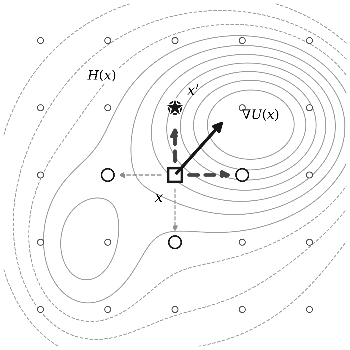
Figure 1:Gradient-informed sampling on a discrete state space. The gradient of a differentiable extension provides local geometric information at the current state , which induces different proposal weights over its Hamming-one neighbourhood . The starred state represents a draw from this proposal. Adapted from Grathwohl et al. (2021).
This can be computed quickly by viewing the update as the selection of a coordinate to modify. In the binary case, this update is always a bit flip. Here, normalises a vector of real-valued scores into probabilities, and denotes the categorical distribution with those probabilities. The resulting proposal is
The categorical case requires selecting both a coordinate and its proposed category. Let denote the current category of coordinate . We represent each categorical coordinate by a one-hot vector when evaluating the gradient. For every alternative category , define the approximate log-probability difference
The first term measures the local effect of assigning category to coordinate , while the second corresponds to its current category.
There are possible coordinate–category updates. We define a categorical proposal over these updates by
After sampling , the proposed state is obtained by changing coordinate from to and leaving all other coordinates unchanged. The full categorical procedure is given in Algorithm 1.
Because the gradient-based proposal uses a first-order approximation and is generally asymmetric, it does not by itself preserve the target distribution. We therefore apply the standard Metropolis–Hastings acceptance correction, described in Section Metropolis–Hastings, which ensures that the target distribution is invariant. Under the ergodicity conditions stated above, the resulting Markov chain converges to the target distribution.
Discrete Langevin Proposal
Gibbs-With-Gradient can outperform uninformed single-coordinate proposals by using the gradient to prioritise promising updates. Its Hamming-one restriction also keeps the Taylor approximation local, but only one coordinate can change per iteration, which may produce strongly correlated samples in high dimensions. Zhang et al. (2022) addresses this limitation with the Discrete Langevin Proposal (DLP), which retains gradient-based directionality while adding a distance penalty that permits multiple coordinates to be proposed simultaneously.
In the running binary example, Gibbs-With-Gradient proposes at most one bit flip, whereas DLP constructs a proposal for every bit and may change several bits in the same iteration.
To derive the proposal, consider the discrete analogue of a Gaussian random-walk kernel,
Combining this kernel with a first-order approximation of the locally balanced weight gives the DLP
The linear term in Equation (17) favours moves predicted to increase , while the quadratic term penalises moves far from the Taylor expansion point. The step size controls the strength of this penalty.
Because the state space factorises as and the exponent in Equation (17) is a sum of coordinate-wise terms, the proposal factorises as . Each factor is the categorical distribution
Thus, larger values of permit more distant proposals, whereas smaller values concentrate the proposal near the current state.
While this may look similar to the proposal formula for Gibbs with Gradient, it is important to note that in DLP, the softmax is computed per coordinate over the potential classes that can be realised. In Gibbs with Gradient, the softmax is over the entire sample to pick only one coordinate. This allows for the parallel update of all coordinates.
The factorisation makes it possible to propose all coordinates in parallel after one gradient evaluation. Although the proposal factors coordinate-wise conditional on the current state, the gradient of the joint log density still guides each coordinate using information from the full current configuration. A Metropolis–Hastings correction can then account for the remaining approximation error and dependence structure. Figure 2 contrasts this parallel update with the single-coordinate update used by Gibbs-With-Gradient.
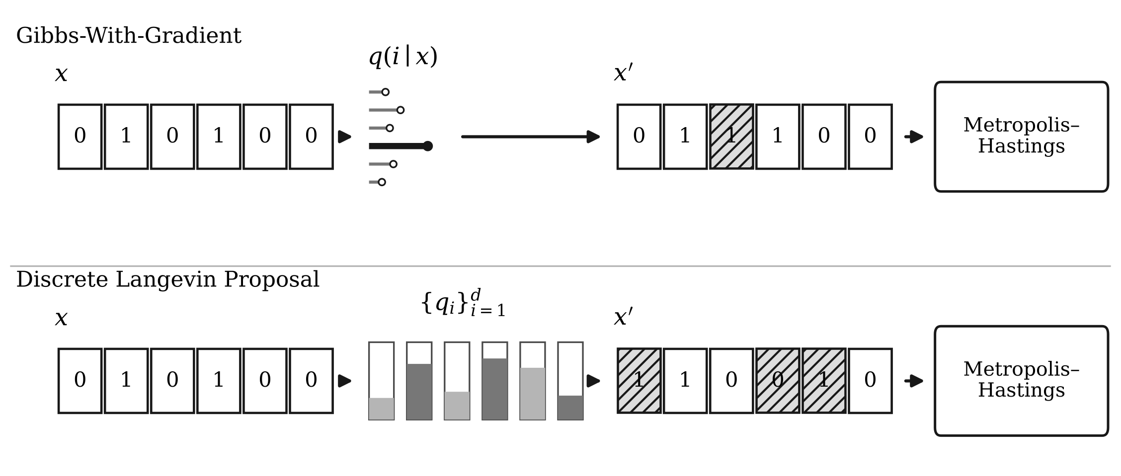
Figure 2:Comparison of gradient-based discrete proposals. Gibbs-With-Gradient samples one coordinate from and proposes a state that differs in that coordinate. The Discrete Langevin Proposal constructs coordinate-wise distributions and can propose several changes in parallel. The displayed Metropolis–Hastings correction gives the adjusted variants; omitting it yields DULA in the discrete Langevin case. Based on Grathwohl et al. (2021) and Zhang et al. (2022).
Using DLP yields two samplers: the discrete Metropolis-adjusted Langevin algorithm (DMALA), which includes a Metropolis–Hastings correction, and the discrete unadjusted Langevin algorithm (DULA), which omits it. DULA generally has asymptotic bias. For log-quadratic targets, however, Zhang et al. (2022) show that this bias vanishes as ; they also bound the bias for targets whose gradients are close to those of a log-quadratic distribution.
In terms of implementation, the cost difference between DULA and DMALA is negligible: while DMALA incorporates a Metropolis–Hastings correction that requires the computation of both and , caching means that only one new proposal distribution is computed per step after initialisation. The cached version of DMALA is given in Algorithm 2.
The core logic lies in the fact that the of the current iteration is either rejected or becomes the for the next sampling step. In the case of rejection, the proposal function does not change as remains the same. In the case of acceptance, the proposal step simply gets updated to match the updated by using , since this proposal must be computed anyway for the accept/reject step. Thus at each step, only one proposal function must be computed.
Beyond Locally Balanced Proposals
Locally balanced proposals offer a convenient framework for incorporating gradients into discrete samplers, but their defining approximation concerns the small-scale limit . At finite scales, local proposals may take a long time to move between separated modes, necessitating longer chains or multiple chains.
For example, if the binary target places high probability on two configurations separated by many low-probability intermediate states, a sequence of single-bit proposals may struggle to move from one mode to the other.
This motivates proposals designed for non-local movement. Zanella (2020) already considers , calling the resulting proposal the naively informed choice because it has the form . Building on this observation, Sun et al. (2023) formalise the large-scale interpretation: they call a proposal family globally balanced if the invariant distribution of its uncorrected informed proposal converges to as . They assume that the base kernel becomes uniform in this limit. Since a state-independent constant cancels in the normalisation of the informed proposal, they write this limit as ; for a normalised kernel on a finite state space, the corresponding limit is . For , the limiting proposal is then
Thus the proposal becomes an independent draw from the target itself and is globally balanced in the sense of Sun et al. (2023). Notice that does not satisfy the locally balanced identity ; local and global balance refer to different limiting regimes.
Any-scale Balanced Sampler
The any-scale balanced sampler introduced by Sun et al. (2023) makes two distinct modifications for proposals outside the local regime. First, it adjusts the density-ratio weighting to match the proposal scale. The family , with , interpolates between the locally balanced choice as and the globally balanced choice as . This scale-dependent relationship is illustrated schematically in Figure 3(a).
Adjusting changes how strongly the proposal favours high-density candidates, but it does not reduce the error in a first-order approximation of . The method therefore makes a second modification: it introduces a quadratic approximation intended to remain informative over larger moves. The log-density difference is approximated by
where is a symmetric matrix shared across states. Setting would recover the usual second-order Taylor approximation locally, but repeatedly computing a Hessian is expensive. Instead, the sampler estimates a global from pairs collected during burn-in:
Thus is fitted to explain observed changes in the gradient and acts as a global curvature approximation. Scale-dependent balancing and curvature approximation address different problems: controls the density-ratio weighting, whereas improves the approximation used to score non-local candidates.
Substituting the quadratic approximation in Equation (21) and into the informed proposal gives
The quadratic term captures cross-coordinate interactions, but it also prevents direct coordinate-wise sampling. Sun et al. (2023) therefore introduce an augmented proposal with a Gaussian auxiliary variable. The augmented construction is used directly with the Metropolis–Hastings correction below.
Choose a diagonal positive semi-definite matrix such that is positive semi-definite, and draw
The matrix square root can be computed by an eigendecomposition or Cholesky factorisation. Conditional on , define
and sample from this distribution. Because is diagonal and the state space factorises, this conditional proposal factorises across coordinates. Equations (23) and the augmented proposal express, respectively, the motivating quadratic approximation and the auxiliary-variable transition implemented by the sampler. The Metropolis–Hastings step accounts for the resulting augmented proposal exactly.
The Metropolis–Hastings acceptance probability for the augmented proposal is
The diagonal matrix controls the conditional proposal variance. Sun et al. (2023) consider two semidefinite programs for choosing it. The AB-max variant minimises the largest eigenvalue of :
This criterion focuses on the worst spectral direction. The AB-trace variant instead solves
The motivation for this objective comes from the continuous quadratic surrogate studied by Sun et al. (2023) in the special case and . In that surrogate, the covariance of the proposal increment is , so minimising the trace of encourages dispersion across coordinates. This covariance identity does not hold literally for the general discrete categorical proposal, whose dispersion also depends on , , and the state space. The authors report that AB-trace performs better empirically and use it as their preferred variant.
The proposal parameters and are correlated and target-dependent. Sun et al. (2023) therefore adapt them by alternating coordinate-wise updates that seek to maximise the empirical average jump distance. For one parameter type , let denote its current value and define the feasible sets and . With the other parameter held fixed, the adaptation block compares with feasible multiplicative perturbations of it over three consecutive chain segments, as shown in Algorithm 3.
The three segments in Algorithm 3 are consecutive: the second begins from and the third from . The full adaptation alternates a block for and a block for . If neither parameter changes during an outer iteration, the update rate is reduced geometrically, for a decay factor ; otherwise the selected parameter values are retained for the next iteration. Because adaptation based on short-run jump distances can be noisy during early mixing, this procedure is intended for burn-in rather than continued adaptation after samples are retained for inference.
Through the combination of a quadratic approximation of the log-probability difference and the adaptive scheme for and , the any-scale sampler interpolates between locally and globally balanced proposals.
Automatic Cyclical Sampling
One common issue with gradient-based samplers for continuous spaces is exploration: as the gradient points in the direction of the closest mode, it gives no information regarding further, more distant modes. This can hinder the accuracy of the sampler in terms of approximating the target distribution.
The same problem applies to gradient-based discrete samplers. Unlike a continuous state space, a discrete space has no arbitrarily small non-trivial perturbations: even the most local move must change at least one coordinate. This granularity can make the trade-off between conservative, high-acceptance moves and larger exploratory moves especially pronounced. Interpolating between locally and globally balanced proposals is therefore a natural way to vary the proposal scale when large movements may be required to escape a local mode.
In the continuous case, many approaches have been proposed for handling the mode-escape problem. One popular approach is cyclical SG-MCMC, discussed in Chapter Stochastic gradient MCMC. A cyclical schedule gradually reduces the step-size of a gradient-based sampler from very large magnitudes to small magnitudes and repeats for several cycles. The large steps at the beginning allow for more exploratory movements, which enable mode discovery; and the smaller step-sizes at the end of the cycle allow for exploitation of the mode. The repetition of the cycles allows for the discovery and exploitation of many modes, which is required for effective characterisation of multi-modal distributions.
Building on this intuition, Pynadath et al. (2024) introduce a sampler that cycles jointly through step sizes and balancing exponents. Varying alone can produce poorly balanced proposals and low acceptance probabilities, so the method uses the generalised DLP
Setting in Equation (29) recovers the standard DLP. Within each cycle, large values of are paired with values of closer to 1 to encourage global exploration; as decreases, moves towards and the proposal becomes more local.
The automatic tuning procedure begins with user-specified endpoint exponents and and a target acceptance rate. Short burn-in runs determine corresponding endpoint step sizes and . These endpoints define the cyclical step-size schedule, following the continuous-space construction of Zhang et al. (2020).
For each step size , the corresponding is selected to maximise an empirical acceptance-rate objective subject to . This monotonic constraint reflects the transition from large moves with more globally balanced weighting at the beginning of a cycle to small, locally balanced moves at its end, while reducing the cost of searching for the full schedule. Figure 3(b) shows the coupled schedules used to move repeatedly from global exploration to local characterisation.
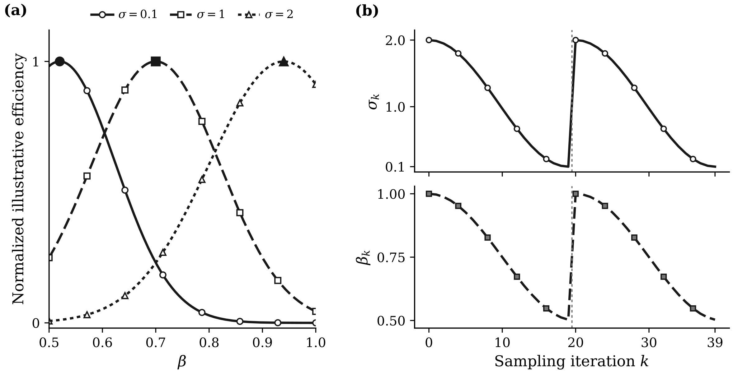
Figure 3:Proposal scale, balancing, and cyclical scheduling. Panel (a) schematically illustrates that the preferred balancing exponent increases with the proposal scale: small-scale proposals favour near , whereas larger-scale proposals favour values closer to 1. The curves show normalised illustrative efficiency rather than empirical measurements. Panel (b) shows coupled schedules for and over two cycles, progressing from large proposals with more globally balanced weighting to small, locally balanced proposals within each cycle. Panel (a) is adapted conceptually from Sun et al. (2023); panel (b) is adapted from Pynadath et al. (2024).
Conclusion
Gradient information can make sampling in high-dimensional discrete spaces substantially more efficient, even though the state space itself is not differentiable. Locally balanced proposals provide the organising principle: they combine an uninformed local kernel with target-specific information and use a Metropolis–Hastings correction to retain the desired target distribution. Gibbs-With-Gradient uses a first-order approximation to choose an informed single-coordinate update, whereas DLP factorises a Langevin-like proposal so that many coordinates can be proposed in parallel.
The appropriate proposal depends on the scale of movement required. Small, locally balanced moves can characterise a mode accurately but may mix slowly between separated modes. Any-scale balancing adapts the balancing exponent and adds a global curvature approximation for more effective non-local moves. Automatic cyclical sampling instead repeats a schedule from large exploratory proposals to small exploitative proposals, pairing each step size with a suitable balancing exponent.
In the running binary example, this progression moves from informed single-bit proposals, through parallel multi-bit updates, to methods that adapt the scale and weighting of those updates to improve movement between separated modes.
These methods trade additional structure and tuning for improved exploration. Their practical performance depends on the quality of the differentiable extension of , the accuracy of the local or quadratic approximation, and the cost of evaluating reverse proposals in the Metropolis–Hastings correction. The adjusted variants provide asymptotically exact sampling under the usual irreducibility and aperiodicity conditions; unadjusted variants can be cheaper, but generally introduce stationary bias.
- Zanella, G. (2020). Informed Proposals for Local MCMC in Discrete Spaces. Journal of the American Statistical Association, 115(530), 852–865.
- Grathwohl, W., Swersky, K., Hashemi, M., Duvenaud, D., & Maddison, C. (2021). Oops I Took A Gradient: Scalable Sampling for Discrete Distributions. In M. Meila & T. Zhang (Eds.), Proceedings of the 38th International Conference on Machine Learning (Vol. 139, pp. 3831–3841). PMLR.
- Zhang, R., Liu, X., & Liu, Q. (2022). A Langevin-like Sampler for Discrete Distributions. In K. Chaudhuri, S. Jegelka, L. Song, C. Szepesvari, G. Niu, & S. Sabato (Eds.), Proceedings of the 39th International Conference on Machine Learning (Vol. 162, pp. 26375–26396). PMLR.
- Sun, H., Dai, B., Sutton, C., Schuurmans, D., & Dai, H. (2023). Any-scale Balanced Samplers for Discrete Space. The Eleventh International Conference on Learning Representations, ICLR 2023, Kigali, Rwanda, May 1-5, 2023.
- Pynadath, P., Bhattacharya, R., Hariharan, A., & Zhang, R. (2024). Gradient-based Discrete Sampling with Automatic Cyclical Scheduling. In A. Globerson, L. Mackey, D. Belgrave, A. Fan, U. Paquet, J. Tomczak, & C. Zhang (Eds.), Advances in Neural Information Processing Systems (Vol. 37, pp. 46728–46763). Curran Associates, Inc.
- Zhang, R., Li, C., Zhang, J., Chen, C., & Wilson, A. G. (2020). Cyclical Stochastic Gradient MCMC for Bayesian Deep Learning. 8th International Conference on Learning Representations, ICLR 2020, Addis Ababa, Ethiopia, April 26-30, 2020.