Introduction to sampling
Introduction
The fundamental objective of Bayesian statistics is to compute the posterior distribution of a random variable given data . In the context of supervised learning, where the data comprises features/inputs and responses/labels , Bayes’ formula for the parameter posterior distribution takes the following form
where denotes the likelihood of observations for the target given inputs , is the density of the prior distribution for , and
denotes the model evidence of the data. Note that, in general the posterior is often only known up-to a normalizing constant, because, aside from simple models, calculating the integral in the model evidence is not feasible for high-dimensional nor is it often available in closed form. Therefore, it is more common to work with the unnormalized posterior .
We note that the ultimate goal in solving (1) is estimating the posterior predictive for new inputs , i.e. the pushforward of the posterior through the test likelihood:
This is a distributed quantity that incorporates both epistemic and aleatoric uncertainty (uncertainty caused by a lack of data or knowledge, respectively), but often we content ourselves with its expectation as a point estimator :
Simulating or sampling from , or from , or for some point estimator is not considered explicitly in this chapter, although it is worth noting that the posterior predictive is often better behaved than the parameter posterior. One primary reason for this may be that it eliminates the non-identifiability arising from exchangeability of the weights on a given layer.
For the remainder of this chapter, we will consider sampling from a generic target distribution , where may or may not be known. The reader can think of as the posterior already introduced in (1), but where we drop the data for notational convenience.
Monte Carlo
The most fundamental sampling algorithm is the Monte Carlo algorithm Robert & Casella, 1999, and it is the basis for many other sampling schemes. Monte Carlo works as follows. Suppose we have a random variable from a distribution which is continuous on . Let be the probability density function for and assume that we are able to simulate independent and identically distributed (i.i.d.) samples from . Note that we may refer to as the distribution itself. For some function of interest , which is integrable with respect to , we wish to estimate an expectation
which is often not available in closed form. Quadrature methods Davis & Rabinowitz, 1984 are suitable in low parameter dimension , and with tricks up to Genz & Malik, 1980 or even Bungartz & Griebel, 2004. However, for large , Monte Carlo reigns supreme due to its remarkable ability to achieve a mean square error (MSE), defined as , that decays at the canonical rate in the number of samples , regardless of dimension or smoothness of the quantity of interest .
The Monte Carlo method is extremely simple to use. We wish to generate independent samples as shown in Algorithm 1.
Using the Monte Carlo samples from , we can estimate the expectation as follows
This beautiful equation has remarkable convergence properties, and it is this gold standard that we aim to achieve with other sampling algorithms. Since the samples are i.i.d. from , and writing , we have
Thus is an unbiased estimator of the target integral. Moreover, we can increase the accuracy of our estimator by increasing the number of samples . By the strong law of large numbers, if , we can guarantee that the Monte Carlo estimator converges almost surely to the true value as the number of samples grows without bound. Formally,
That is, with probability one the estimator will eventually get arbitrarily close to the truth. If we invoke the central limit theorem, then we can also quantify how accurate is for a given finite . Define the variance
and assume . Then as ,
Equivalently, for large ,
so that the standard error of the Monte Carlo estimator is and its MSE decays at the canonical rate (i.e. root‐MSE ). This convergence is independent of the dimension or smoothness of , and is the benchmark against which all more advanced sampling methods are compared.
Often, a challenge is that we cannot sample from our target probability distribution directly, and can only evaluate or sample from a non-negative unbiased estimator of . Addressing these challenges has led to the development of the algorithms presented in the remainder of this chapter.
Rejection Sampling
Suppose that is a probability density function from which we can sample relatively easily and that is the target density from which we would like to sample. Suppose in addition that there exists a constant, , such that
whenever . Then, we can formulate an algorithm for simulating samples from as given in Algorithm 2.
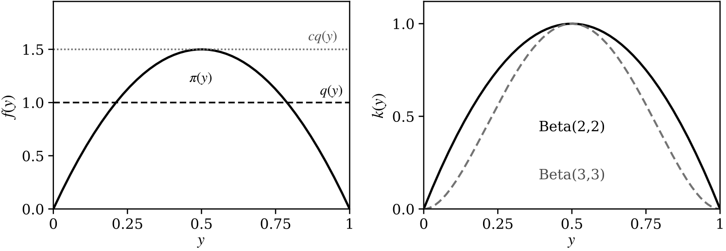
Figure 1:Rejection sampling from a Beta target using a uniform proposal . Left: alone does not dominate , but the envelope with does. Right: the acceptance probability , shown also for a Beta target (), for which acceptance is lower.
This algorithm is referred to as rejection sampling. We can see that this recipe will be very computationally efficient if the densities and are approximately equal and the constant can be chosen close to 1. In this case, the acceptance probability will generally be close to 1. On the other hand, if and are very different, then many runs of the algorithm may be required before a value is finally accepted.
Despite its attraction of ease of implementation and simulation, the efficiency of rejection sampling relies on (i) having a good proposal distribution and (ii) a bound . Note that it can easily be modified to work with only , but these difficulties remain.
Importance Sampling
The importance sampling estimator of begins by re-writing the integral as follows
where is a density such that , whenever . We now produce i.i.d. samples from , and estimate
We call this procedure importance sampling. The density is called the proposal or instrumental density and are the* importance weights*. Note that is an unbiased Monte Carlo estimator of , as shown in Equation (7). There are two reasons why we might be interested in performing importance sampling:
Sampling from is not possible or too expensive.
The function has a large variance, so the conventional unbiased estimator has large Monte Carlo error.
Recalling the results of Section Monte Carlo, the effective test function is now , and so its regularity dictates the convergence behaviour. Hence, if possible, we should choose a proposal density such that the variance of is small. It can be shown that the optimal proposal distribution is , however that does little good by itself, since we are back to the same problem of approximating . However, it can provide useful guidance.
Suppose that we only know how to evaluate . It is easy to see that an unbiased estimator of the normalizing constant can be built using the following identity
It is left as an exercise to the reader to build a consistent (but biased) self-normalized importance sampling estimator using only . Unlike rejection sampling, importance sampling does not waste samples through the rejection step, which could be a high amount depending on the application at hand.
As alluded to already, a major disadvantage of importance sampling is that it can result in high variance. There are numerous methods beyond what has been introduced here to alleviate such issues, including the sequential importance sampling and resampling methods which will be introduced later in Section Sequential Monte Carlo.
Markov chain Monte Carlo
The preceding sections have introduced Monte Carlo integration and two classical approaches—rejection sampling and importance sampling—for drawing samples from a target distribution , typically the posterior in Bayesian inference. While these methods are simple to use and theoretically well-founded, they suffer significant limitations in high-dimensional settings. Rejection sampling becomes increasingly inefficient as the dimension grows, due to the difficulty of finding proposal distributions that tightly bound the target. Importance sampling, although more flexible, tends to suffer from high variance unless the proposal distribution is well matched to the target Agapiou et al., 2017Chatterjee & Diaconis, 2018—a condition that is notoriously hard to satisfy in practice, especially in the multimodal, heavy-tailed, and high-dimensional posteriors encountered in Bayesian deep learning Papamarkou et al., 2024.
Markov Chain Monte Carlo (MCMC) provides a powerful and general framework to overcome these challenges. Rather than attempting to generate independent samples from , MCMC constructs a Markov chain whose stationary distribution is itself. By simulating a trajectory through parameter space in such a way that, asymptotically, the empirical distribution of visited states converges to the target, MCMC transforms the task of independent sampling into one of designing a suitable transition mechanism that ensures both* ergodicity* and* invariance* with respect to Tierney, 1994.
In practical terms, MCMC methods produce a correlated sequence of samples , which, under suitable conditions, can still be used to approximate expectations under using ergodic averages. The canonical estimator takes the form:
which, despite the dependence between samples, converges to the true posterior expectation under mild regularity assumptions Geyer, 2011.
In what follows, we introduce several fundamental MCMC algorithms, starting with the Metropolis–Hastings algorithm, which provides a generic recipe for constructing -invariant Markov chains from arbitrary proposal distributions Metropolis et al., 1953Hastings, 1970. We then examine key special cases—random-walk Metropolis, the Metropolis-adjusted Langevin algorithm (MALA), and Hamiltonian Monte Carlo (HMC)—that are particularly relevant in the context of high-dimensional posterior inference in Bayesian deep learning. Throughout, we pay close attention to algorithmic trade-offs, scaling behaviour Roberts et al., 1997Roberts & Rosenthal, 1998Fearnhead et al., 2025, and diagnostic tools for assessing convergence and sampling efficiency Brooks & Gelman, 1998.
Metropolis–Hastings
Markov chain Monte Carlo (MCMC) proceeds by generating a Markov chain with transition kernel , described by a density on , which is invariant with respect to the target posterior :
The Metropolis–Hastings (MH) algorithm achieves this invariance by first choosing an arbitrary proposal density that proposes given the current iterate of the Markov chain , and then accepting or rejecting each proposed move so that detailed balance—and hence (19)—holds.
Concretely, we can define the MH transition kernel as
where the acceptance probability is
Because , any unknown normalisation cancels and only the unnormalized density is needed. See Algorithm 3 for a full implementation.
Invariance with respect to is a necessary condition for building convergent estimators from a Markov chain. The chain also needs to have certain other stability properties, collectively known as ergodicity, to ensure empirical averages (6) built from its output converge. A desirable and achievable property is called* geometric ergodicity*, which essentially guarantees linear convergence, i.e. the dependence on the initial condition vanishes geometrically.
Random walk Metropolis
A particularly simple—and historically important—special case of the Metropolis–Hastings algorithm is the random–walk Metropolis (RWM) proposal, in which one sets
where is any symmetric density, . The canonical choice is
so that , i.e. . Due to symmetry, the Metropolis acceptance probability simplifies to
Local moves and tuning. RWM proposals are inherently local: each candidate lies in a neighbourhood of . If is too small, the chain makes only tiny steps and mixes very slowly; if is too large, most proposals fall in low-density regions and are rejected. Optimal scaling results show that, for a wide class of -dimensional targets, the stationary acceptance rate tends to as when Roberts et al., 1997. In practice, one therefore adapts so that the empirical acceptance rate lies between about and .
Preconditioning. When components of have very different scales or strong correlations, one can replace by , where is a positive-definite “preconditioning” matrix (often an estimate of the posterior covariance). This preconditioned RWM retains symmetry and thus the same simplified acceptance probability, but can yield orders-of-magnitude improvements in computational efficiency, i.e. less samples required to sample the target, because the proposed parameters will be more closely aligned with the posterior distribution, and thus less likely to be rejected.
Gibbs Sampler
Given a multi-variate , it may be intractable to sample all at once. However if the full conditional distributions for each coordinate are known, then it becomes possible to apply Gibbs sampling.
The Gibbs sampling algorithm is fairly straightforward. Given the proposals are known, the Gibbs algorithm updates the sample by updating each coordinate one at a time, i.e. , where denotes all coordinates except . While it may be tempting to update all coordinates at the same time, this would not properly preserve the joint distribution as all coordinates would be updated independently. We include a simple formulation in Algorithm 4.
Given that the Gibbs sampler is drawing from the correct proposal, the typical Metropolis-Hastings acceptance step is not needed in this case. However, this sampler suffers from slow and highly correlated samples due to the nature of the single coordinate update approach.
It is possible to extend the initial Gibbs sampler to a block-style approach in the case where the joint distribution over multiple coordinates is known. Instead of the single-coordinate marginal, if we know the joint distribution over one-set of coordinates conditioned on another set, it is possible to quickly sample by alternative sampling from each joint distribution. This is known as the Block-Gibbs sampler. More formally, if we have two sets of coordinates , the block Gibbs sampler proceeds by sampling , and then sampling . This sampling algorithm avoids the pitfalls of the typical Gibbs sampler. However, it is only possible to use this in cases where the conditional distributions over blocks of coordinates is known.
Metropolis-adjusted Langevin Algorithm
The random-walk Metropolis ignores gradient information about . The Metropolis–Adjusted Langevin Algorithm (MALA) rectifies this by using an Euler–Maruyama discretisation of the overdamped Langevin diffusion
where is standard Brownian motion on , and whose stationary law is . Concretely, the MALA proposal is
This drift term biases proposed moves towards regions of higher posterior density, enabling larger step-sizes than RWM and better acceptance rates. The MALA proposal also forms the basis for many other wonderful Monte Carlo algorithms, including the stochastic gradient Langevin dynamics (SGLD) Welling & Teh, 2011 and all other stochastic gradient MCMC (SG-MCMC) algorithms, which will be the focus of the next chapter.
Gradient-based tuning. Under regularity conditions, choosing yields an optimal stationary acceptance rate of approximately 0.574 as Roberts & Rosenthal, 1998. In applications, one often adapts to target an acceptance rate of about to . This can be done by monitoring the acceptance rate and adjusting accordingly, or by using more sophisticated adaptive schemes that adjust the step size based on the empirical gradient information.
Preconditioned MALA and robustness. Analogous to RWM, one can introduce a symmetric preconditioning matrix , replacing by both in the covariance and in the drift:
Preconditioning often dramatically accelerates convergence on anisotropic posteriors. However, because MALA relies on , it can be sensitive to regions where the gradient is large or ill-behaved (e.g. lighter-than-Gaussian tails). Common mitigations include gradient clipping or fallback to RWM outside of a “trust region.”
Monitoring Performance
Assessing the quality of an MCMC run is essential to ensure that empirical averages reliably approximates . Three widely used diagnostics are:
1. Autocorrelation and Integrated Autocorrelation Time. For a scalar summary of , define the lag- autocorrelation
As the Markov chain is stationary, , and as . The slower decays, the more correlated is the chain. One can show that, via the Markov-chain central limit theorem,
The quantity is the integrated autocorrelation time, and the* effective sample size* measures the number of independent draws represented by correlated samples. Figure Figure 3 illustrates autocorrelation decay. A related metric is the* expected squared jumping distance* (ESJD) , which balances move size against acceptance rate. Larger moves will reduce the correlation between elements of the Markov chain, however, larger moves are also less likely to be accepted, which means that the chain does not evolve. Therefore, the challenge for practitioners, is to balance between small moves (high correlation and high acceptance rate) and large moves (low correlation and low acceptance rate).
2. Trace Plots. Plotting the sequence versus iteration provides a simple-to-interpret visual representation of mixing and stationarity. Well‐mixed chains rapidly traverse the bulk of the posterior, showing no apparent trends or “stickiness” (see Left Panel Figure Figure 2). Conversely, slow mixing or multimodality is signalled by long periods of drift or entrapment in subregions of the posterior (see Right Panel Figure Figure 2). Trace plots are a useful visual tool for diagnosing the efficiency of an MCMC algorithm, however, they tend to be most useful for low-dimensional posteriors as it is easier to visualise all of the parameters , whereas, for high-dimensional posteriors, visualising all of the parameters in the Markov chain individually is often impractical.
3. Potential Scale Reduction (Gelman–Rubin) Diagnostic. When multiple chains are run from overdispersed starting points, one can compare the between-chain variance to the* within-chain variance* . The* potential scale reduction factor*
tends to 1 as all chains converge to the same target distribution Gelman & Rubin, 1992. Values of are commonly taken to indicate satisfactory convergence, after which samples from all chains may be pooled to produce an approximation to the posterior .
In practice, one would usually employ a combination of these diagnostics: trace plots for qualitative assurance, autocorrelation and ESS for quantitative accuracy, and to guard against failure to explore multimodal targets.
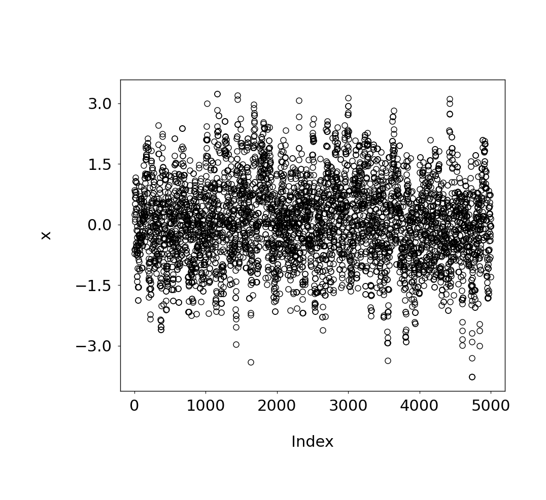
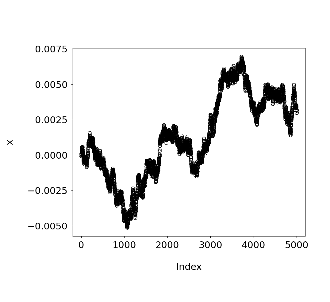
Figure 2:Trace plots for (left) and (right).
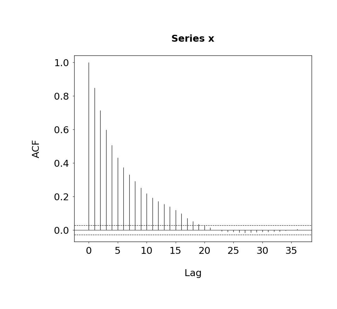
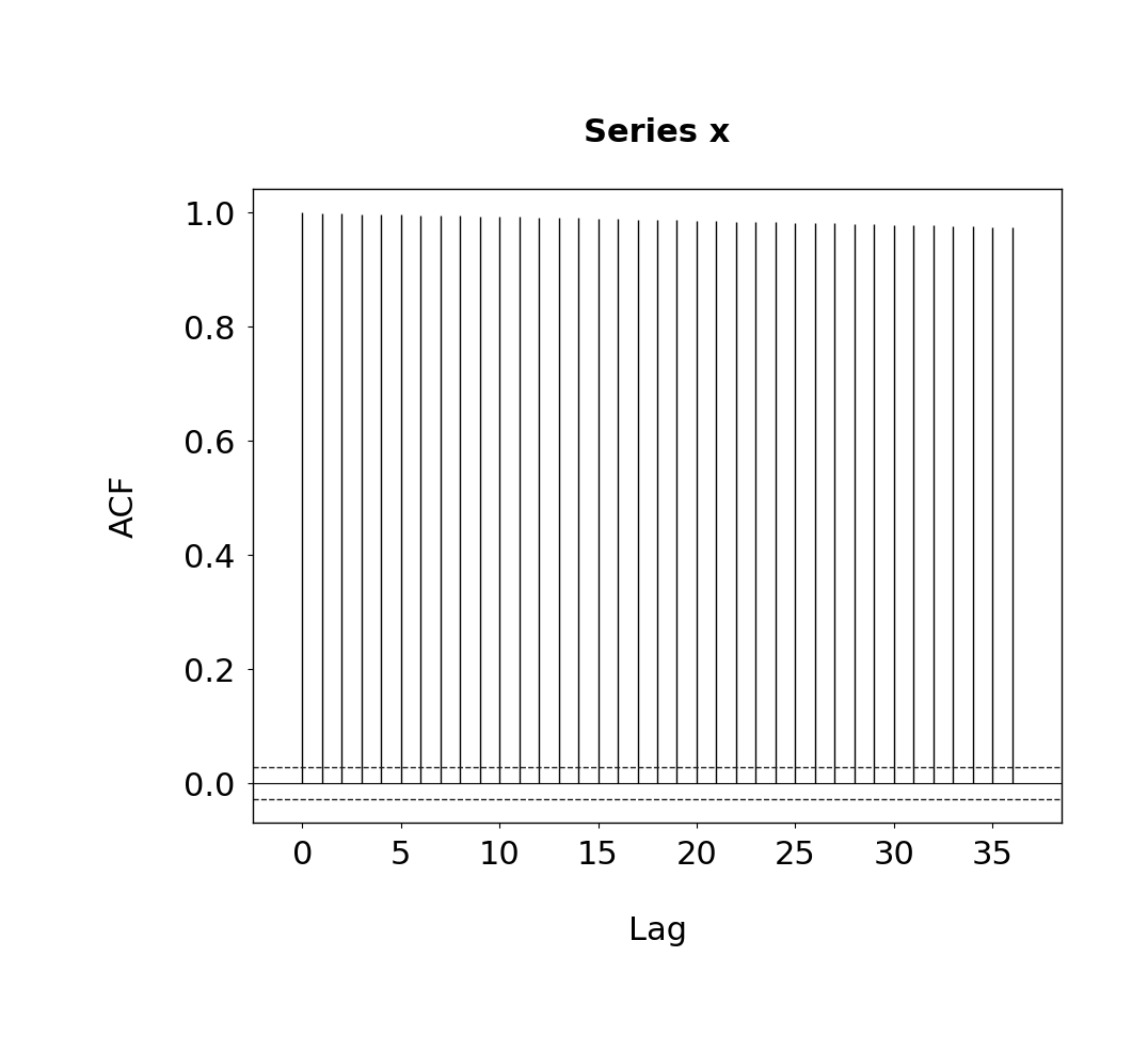
Figure 3:Corresponding ACFs for (left) and (right).
Hamiltonian Monte Carlo
Random–walk Metropolis (RWM) requires proposal steps of size to maintain a non–degenerate acceptance rate in dimension , whereas MALA can take steps of size . Hamiltonian Monte Carlo (HMC) goes a step further: with an integration step size it still enjoys an acceptance rate bounded away from 0 while exploring much larger regions of parameter space between consecutive accept–reject decisions Beskos et al., 2013Duane et al., 1987Neal, 2011Cobb & Jalaian, 2021. The key is to embed the ‐dimensional parameter in a -dimensional* phase space* and simulate approximate Hamiltonian dynamics that preserve a surrogate “total energy”.
Extended target and Hamiltonian. Introduce an auxiliary momentum variable and a positive–definite* mass matrix* . Define the Hamiltonian
so that the joint density has marginal and independent .
Hamiltonian dynamics. The continuous equations of motion are
which conserve exactly and therefore move along surfaces of constant joint density. Exact simulation is impossible for general targets , so HMC uses the second–order, symplectic leapfrog integrator Leimkuhler & Reich, 2005 with step size :
One repeats this map times, with and is the integration time.
HMC kernel. Starting from :
Draw momentum .
Apply leapfrog steps (36) to obtain .
Accept with probability
Set if accepted, otherwise ; discard .
Because the leapfrog map is volume–preserving (i.e. the Jacobian ) and symmetric (its inverse is obtained by and running the steps backward), the Metropolis correction guarantees is invariant; the posterior is therefore stationary for the marginal chain on .
High‐dimensional scaling. For product targets with , one can show Fearnhead et al., 2025 that to keep a well-behaved acceptance rate, one must scale , hence . The computational cost per effectively independent draw is therefore , compared with for MALA and for RWM.
Practical tuning.
Step size . During warm–up, adapt (e.g. with dual‐averaging) to target an acceptance rate in the range; theory suggests is asymptotically optimal Beskos et al., 2013.
Trajectory length . Too small gives RWM‐like behaviour; too large wastes computation and may return to near the starting point. Popular heuristics randomise or employ the No‐U‐Turn criterion Hoffman & Gelman, 2014.
Mass matrix . Setting to an estimate of the posterior covariance (or its diagonal) acts like the preconditioning matrices used with RWM and MALA, dramatically improving convergence when parameters are on different scales.
Because HMC combines long, momentum‐driven proposals with high acceptance probabilities, it has become the default sampler in many Bayesian deep‐learning applications, where posteriors are high‐dimensional, strongly correlated and feature narrow valleys that thwart simpler MCMC methods.
Sequential Monte Carlo
Sequential Monte Carlo (SMC) methods are a set of Monte Carlo algorithms designed to sample from a sequence of target probability densities of increasing dimension, where each one is defined on the product space Doucet et al., 2001Del Moral, 2004. This is referred to as the smoothing distribution in the context of state-space models. Often one may be interested only in the time marginal , which is known as the* filtering distribution*. Suppose
where the un-normalized density admits the decomposition
and and can be evaluated, and is the unknown normalizing constant given by
Note that we write
SMC provides an approximation of and an estimate of at time 1 then an approximation of and an estimate of at time 2 and so on. The approximations are done sequentially in time:
At time step 1, one samples samples from some given function and then approximates and using these samples;
At time step 2, sample from some function , and use the cumulative samples to approximate and .
Consider another probability density that is easy to sample from, and such that the support of includes the support of . Then, we have the following importance sampling (IS) identities
where is the unnormalized weight function and in light of (39) we have the following recursive definition of the weights
Assume we draw, sequentially in time, independent samples , , from (see Algorithm 6). We have the following unbiased estimator of :
A consistent self-normalized importance sampling estimator of , for an arbitrary function , is given by
where
These are the ingredients of the sequential importance sampling (SIS) algorithm, given in Algorithm 6. In Algorithms 6 and 7 we take .
As grows the weights will degenerate, in the sense that one will dominate the rest. This can be monitored by the effective sample size, which is related to the variance of the weights:
One way to mitigate this somewhat is by resampling, i.e. for , let
Resampling slightly increases the variance of the estimator, but the particles are rejuvenated at the filtering end, and under suitable conditions the filter can even remain stable online for infinite time Del Moral, 2004. Note that this branching of the particles forward in time means coalescence backward in time, so the particles still degenerate for small times, which is problematic for the smoother. SIS along with resampling is called sequential importance resampling (SIR) or sequential Monte Carlo (SMC). See Algorithm 7. In the context of a state space model, is often chosen as the forward evolution kernel of the hidden process, and in the filtering context this specific choice is often called the bootstrap particle filter. In practice, one resamples when the ESS is less than a threshold (e.g. or ). See Chopin & Papaspiliopoulos (2020) for a recent comprehensive introduction.
Summary
This chapter introduced the Monte Carlo algorithm and a number of methods that develop it. Each addresses the same underlying difficulty: simulating from, or estimating expectations under, a target distribution that in most applications can only be evaluated up to an unknown normalising constant.
When independent samples from are available, Monte Carlo integration (Section Monte Carlo) applies directly. When they are not, rejection sampling (Section Rejection Sampling) and importance sampling construct estimators from an accessible proposal distribution. Both are exact in principle, but become inefficient in high dimension unless the proposal closely matches the target.
Markov chain Monte Carlo (Section Markov chain Monte Carlo) removes the need for independent draws by constructing a Markov chain whose stationary distribution is the target. The Metropolis–Hastings algorithm (Section Metropolis–Hastings) provides the general recipe, with the random-walk Metropolis algorithm (Section Random walk Metropolis), the Gibbs sampler, the Metropolis-adjusted Langevin algorithm (Section Metropolis-adjusted Langevin Algorithm), and Hamiltonian Monte Carlo (Section Hamiltonian Monte Carlo) as the special cases treated here. Since the samples are correlated, step-size tuning and the convergence diagnostics of Section Monitoring Performance are essential in practice.
Sequential Monte Carlo (Section Sequential Monte Carlo) extends importance sampling to a sequence of targets on nested product spaces, as in filtering. Sequential importance sampling with resampling propagates weighted particles forward in time, with resampling when the effective sample size drops.
The methods play complementary roles: rejection and importance sampling suit low-dimensional or well-matched problems, MCMC is the standard tool for high-dimensional Bayesian computation, and sequential Monte Carlo is suited to inference along a sequence. These ideas are taken further in the chapters that follow. For example, stochastic gradient MCMC is covered in Chapter Stochastic Gradient MCMC, and sequential Monte Carlo samplers, which applies SMC to an artificial sequence of intermediate targets with MCMC mutations, with tempering and multilevel extensions for neural network posteriors, in Chapter Sequential Monte Carlo samplers.
- Robert, C. P., & Casella, G. (1999). Monte Carlo statistical methods. Springer.
- Davis, P. J., & Rabinowitz, P. (1984). Methods of Numerical Integration (Second Edition). Academic Press.
- Genz, A. C., & Malik, A. A. (1980). Remarks on algorithm 006: An adaptive algorithm for numerical integration over an N-dimensional rectangular region. Journal of Computational and Applied Mathematics, 6(4), 295–302.
- Bungartz, H.-J., & Griebel, M. (2004). Sparse grids. Acta Numerica, 13, 147–269.
- Agapiou, S., Papaspiliopoulos, O., Sanz-Alonso, D., & Stuart, A. M. (2017). Importance Sampling: Intrinsic Dimension and Computational Cost. Statistical Science, 32(3), 405–431.
- Chatterjee, S., & Diaconis, P. (2018). The sample size required in importance sampling. The Annals of Applied Probability, 28(2), 1099–1135.
- Papamarkou, T., Skoularidou, M., Palla, K., Aitchison, L., Arbel, J., Dunson, D., Filippone, M., Fortuin, V., Hennig, P., Hernández-Lobato, J. M., Hubin, A., Immer, A., Karaletsos, T., Khan, M. E., Kristiadi, A., Li, Y., Mandt, S., Nemeth, C., Osborne, M. A., … Zhang, R. (2024). Position: Bayesian Deep Learning is Needed in the Age of Large-Scale AI. In R. Salakhutdinov, Z. Kolter, K. Heller, A. Weller, N. Oliver, J. Scarlett, & F. Berkenkamp (Eds.), Proceedings of the 41st International Conference on Machine Learning (Vol. 235, pp. 39556–39586). PMLR.
- Tierney, L. (1994). Markov Chains for Exploring Posterior Distributions. The Annals of Statistics, 22(4), 1701–1728.
- Geyer, C. J. (2011). Introduction to Markov chain Monte Carlo. Handbook of Markov Chain Monte Carlo, 3–48.
- Metropolis, N., Rosenbluth, A. W., Rosenbluth, M. N., Teller, A. H., & Teller, E. (1953). Equation of State Calculations by Fast Computing Machines. The Journal of Chemical Physics, 21(6), 1087–1092.
- Hastings, W. K. (1970). Monte Carlo sampling methods using Markov chains and their applications. Biometrika, 57(1), 97–109.
- Roberts, G. O., Gelman, A., & Gilks, W. R. (1997). Weak convergence and optimal scaling of random walk Metropolis algorithms. The Annals of Applied Probability, 7(1), 110–120.
- Roberts, G. O., & Rosenthal, J. S. (1998). Optimal scaling of discrete approximations to Langevin diffusions. Journal of the Royal Statistical Society: Series B (Statistical Methodology), 60(1), 255–268.
- Fearnhead, P., Nemeth, C., Oates, C. J., & Sherlock, C. (2025). Scalable Monte Carlo for Bayesian Learning. Cambridge University Press.
- Brooks, S. P., & Gelman, A. (1998). General methods for monitoring convergence of iterative simulations. Journal of Computational and Graphical Statistics, 7(4), 434–455.