Stochastic Gradient MCMC - Handbook of Bayesian Deep Learning

Deep learning models extensively use stochastic gradients (i.e., mini-batches) to reduce the memory requirements of model training Bottou, 1991Shun-Amari, 1993. Under suitable assumptions, stochastic gradients computed from individual samples or minibatches can be used in place of full-batch gradients while retaining almost-sure convergence guarantees. Sebbouh et al., 2021. In this chapter, we introduce stochastic gradient MCMC (SG-MCMC) methods, in which stochastic gradients make MCMC suitable for modern deep learning models.

Introduction¶

Standard MCMC algorithms are asymptotically exact samplers under suitable conditions Hastings, 1970; Chapter Introduction to sampling provides an introduction to MCMC and HMC. For Langevin-based methods, an appropriate decaying step-size schedule yields asymptotic convergence to the target distribution Chen et al., 2015. However, using the entire dataset to compute each update makes full-batch MCMC impractical for deep learning models, which commonly have tens of millions of parameters. Inspired by stochastic gradient descent (SGD), stochastic gradient MCMC (SG-MCMC) uses stochastic gradients to approximate full-batch MCMC updates. Similar ideas have been transferred to mini-batch Metropolis–Hastings (MH) algorithms Korattikara et al., 2014Quiroz et al., 2019Zhang et al., 2020. However, mini-batch MH often relies on strong assumptions, such as bounded log-likelihoods or bounded gradients, which are not guaranteed for deep learning models. SG-MCMC Welling & Teh, 2011Chen et al., 2014Ding et al., 2014 addresses these practical concerns under fewer assumptions and with substantially lower memory requirements, thereby bridging the gap between MCMC and Bayesian neural networks (BNNs).

Classic SG-MCMC Algorithms¶

In this section, we introduce two concrete examples of SG-MCMC algorithms that are widely used for deep learning models.

Notation¶

Let $\theta$ be the parameters of a deep learning model, and let $\mathcal{S}=\{\theta_s\}_{s=1}^{M}$ be a sample set collected during the MCMC process. Due to memory constraints, we can collect only a finite number of samples to characterise the posterior distribution:

p(\theta\mid\mathcal{D}) \approx \frac{1}{M}\sum_{s=1}^{M}\delta(\theta-\theta_s),

(1)

where $\delta(\cdot)$ is the Dirac delta function (also known as the unit impulse) Jeffrey, 1990. At inference time, the sample set is used for Bayesian model averaging (BMA) Chen et al., 2025, in which the predictive probabilities of all collected samples contribute to the final prediction:

\hat{y} = \operatorname*{arg\,max}_{y\in\mathcal{Y}}\mathbb{E}_{\theta\sim p(\theta\mid\mathcal{D})}\left[p(y\mid x,\theta)\right] \approx \operatorname*{arg\,max}_{y\in\mathcal{Y}}\frac{1}{M}\sum_{s=1}^{M}p(y\mid x,\theta_s).

(2)

The goal of each SG-MCMC algorithm is to sample from the posterior distribution and collect such a sample set to reconstruct an approximate posterior distribution.

Stochastic Gradient Langevin Dynamics¶

Stochastic Gradient Langevin Dynamics (SGLD) Welling & Teh, 2011 is the first well-known SG-MCMC algorithm. The full-batch energy function is $U(\theta)=-\sum_{(\bm{x}, \bm{y})\in\mathcal{D}}\log p(\bm{y}\mid\bm{x},\theta)-\log p(\theta)$ . Its mini-batch estimate is

\widetilde{U}(\theta)=-\frac{|\mathcal{D}|}{|\bm{\Xi}|}\sum_{(\bm{x}, \bm{y})\in\bm{\Xi}}\log p(\bm{y}\mid\bm{x},\theta)-\log p(\theta),

(3)

where $\bm{\Xi}\subset\mathcal{D}$ is the sampled batch. The sampling process for SGLD follows the Langevin dynamics:

\theta_{t+1} \gets \theta_t-\alpha_t\nabla_{\theta_t}\widetilde{U}(\theta_t)+\sqrt{2\alpha_t}\,\bm{\epsilon}_t,~~~~\bm{\epsilon}_t \sim \mathcal{N}(\bm{0},\bm{I}),

(4)

where $\alpha_t$ is the step size at iteration $t$ . The complete SGLD framework is outlined in Algorithm 1. Compared with standard SGD, SGLD introduces an additional random-noise term $\sqrt{2\alpha_t}\,\bm{\epsilon}_t$ . As noted by Welling & Teh (2011), SGLD approaches standard unadjusted Langevin dynamics Roberts & Tweedie, 1996 when the step size $\alpha_t$ is sufficiently small, as the injected noise dominates the stochastic-gradient noise. Under standard regularity conditions, convergence is guaranteed by a decaying step-size schedule Bottou, 1999Welling & Teh, 2011Ma et al., 2015. Any schedule satisfying i) $\sum_{t=1}^{\infty}\alpha_t=\infty$ and ii) $\sum_{t=1}^{\infty}\alpha_t^2<\infty$ allows the sampler to explore the target distribution while controlling its asymptotic error Chen et al., 2025. Notably, mini-batch noise in SGD without externally injected noise can produce behaviour qualitatively similar to SGLD, but converges to a biased approximate posterior Mandt et al., 2017.

Algorithm 1 (Stochastic Gradient Langevin Dynamics (SGLD))

Inputs: dataset $\mathcal{D}$ , initial sample $\theta_0 \in \Theta$ , step-size schedule $\{\alpha_t\}_{t\geq 0}$
Output: collected samples $\mathcal{S} \subset \Theta$

$\theta \gets \theta_0$ ; $\mathcal{S} \gets \emptyset$
For each iteration:
1. $\bm{\Xi} \gets$ a mini-batch sampled from $\mathcal{D}$
2. $\widetilde{U} \gets -\frac{|\mathcal{D}|}{|\bm{\Xi}|}\log p(\bm{\Xi}\mid \theta) - \log p(\theta)$ — Note: Compute energy
3. $\theta \gets \theta - \alpha_t \nabla_{\theta} \widetilde{U} + \sqrt{2\alpha_t}\bm{\epsilon}$ — Note: $\bm{\epsilon} \sim \mathcal{N}(\bm{0}, \bm{I})$
4. $\mathcal{S} \gets \mathcal{S} \cup \{\theta\}$

Stochastic Gradient Hamiltonian Monte Carlo¶

Full-batch Hamiltonian Monte Carlo (HMC) has achieved gold-standard performance in Bayesian inference Izmailov et al., 2021. HMC incorporates a kinetic-energy term characterised by a set of auxiliary “momentum” variables. To adapt HMC to deep learning models and reduce its memory requirements, stochastic gradient HMC (SG-HMC) Chen et al., 2014 eliminates the need for full-batch gradients and removes the MH correction used by full-batch HMC. Specifically, naive SG-HMC replaces the full-batch energy in the Hamiltonian with its mini-batch estimate:

\widetilde{H}(\theta,\bm{r})=\widetilde{U}(\theta)+\frac{1}{2}\bm{r}^{\top}\bm{M}^{-1}\bm{r}=-\frac{|\mathcal{D}|}{|\bm{\Xi}|}\sum_{(\bm{x}, \bm{y}) \in\bm{\Xi}}\log p(\bm{y}\mid\bm{x},\theta)-\log p(\theta)+\frac{1}{2}\bm{r}^{\top}\bm{M}^{-1}\bm{r},

(5)

where $\bm{r}$ is the momentum and $\bm{M}$ is a positive-definite mass matrix. Despite its intuitive appeal and simplicity, naive SG-HMC does not preserve the target posterior Chen et al., 2014: stochastic-gradient noise makes the desired joint distribution $\pi(\theta,\bm{r})\propto\exp(-H(\theta,\bm{r}))$ , where $H(\theta,\bm{r})=U(\theta)+\frac{1}{2}\bm{r}^{\top}\bm{M}^{-1}\bm{r}$ , non-invariant. To mitigate this problem, Chen et al. (2014) introduces a “friction” term $C\bm{M}^{-1}\bm{r}$ . If $\widehat{B}$ estimates the stochastic-gradient noise coefficient and $C\geq\widehat{B}$ , the practical dynamics are

\mathrm{d}\theta=\bm{M}^{-1}\bm{r}\,\mathrm{d}t~~~~\text{and}~~~~\mathrm{d}\bm{r}=-\nabla_{\theta}\widetilde{U}(\theta)\,\mathrm{d}t-C\bm{M}^{-1}\bm{r}\,\mathrm{d}t+\sqrt{2(C-\widehat{B})}\,\mathrm{d}\bm{W}_t.

(6)

Here, $\bm{W}_t$ is standard Brownian motion. The friction and injected-noise terms counteract the stochastic-gradient noise. These modified dynamics are commonly known as second-order Langevin dynamics Wang & Uhlenbeck, 1945. The complete SG-HMC framework is outlined in Algorithm 2.

Algorithm 2 (Stochastic Gradient Hamiltonian Monte Carlo (SG-HMC))

Inputs: dataset $\mathcal{D}$ , initial sample $\theta_0 \in \Theta$ , initial momentum $\bm{r}_0$ , step-size schedule $\{\alpha_t\}_{t\geq 0}$ , inner steps $m$ , friction coefficient $C$ , noise estimate $\widehat{B}$
Output: collected samples $\mathcal{S} \subset \Theta$

$\theta \gets \theta_0$ ; $\bm{r} \gets \bm{r}_0$ ; $\mathcal{S} \gets \emptyset$
For each iteration:
1. $\bm{r} \sim \mathcal{N}(\bm{0}, \bm{M})$ — Note: Optionally resample momentum
2. $(\theta^{(0)}, \bm{r}^{(0)}) \gets (\theta, \bm{r})$
3. For $i = 1$ to $m$ :
  1. $\bm{\Xi} \gets$ a mini-batch sampled from $\mathcal{D}$
  2. $\widetilde{U} \gets -\frac{|\mathcal{D}|}{|\bm{\Xi}|}\log p(\bm{\Xi}\mid \theta^{(i-1)}) - \log p(\theta^{(i-1)})$ — Note: Compute energy
  3. $\theta^{(i)} \gets \theta^{(i-1)} + \alpha_t \bm{M}^{-1}\bm{r}^{(i-1)}$
  4. $\bm{r}^{(i)} \gets \bm{r}^{(i-1)} - \alpha_t \nabla_{\theta} \widetilde{U} - \alpha_t C \bm{M}^{-1} \bm{r}^{(i-1)} + \sqrt{2\alpha_t(C-\widehat{B})}\bm{\epsilon}_t$ — Note: $\bm{\epsilon}_t \sim \mathcal{N}(\bm{0}, \bm{I})$
4. $(\theta, \bm{r}) \gets (\theta^{(m)}, \bm{r}^{(m)})$ — Note: No Metropolis-Hastings step
5. $\mathcal{S} \gets \mathcal{S} \cup \{\theta\}$

Practical Concerns and Recent Improvements¶

SG-MCMC methods have been shown to be effective on many small-scale deep learning models Welling & Teh, 2011Chen et al., 2014Ding et al., 2014. However, their application to large-scale deep learning is hindered by several practical concerns. In this section, we discuss these concerns and selected attempts to address them. Chapter Low-precision sampling presents a complementary perspective on scalable, low-precision sampling.

Sampling from Diverse Local Minima¶

The loss surface (or energy landscape) of deep learning models is highly non-convex and multimodal Li et al., 2018Zhang et al., 2020, which makes it difficult for sampling algorithms to move between modes. Moreover, a loss surface typically contains multiple local minima that may all represent good solutions. However, traditional SG-MCMC samplers commonly use a decaying step size and converge to only one local minimum, reducing their ability to explore the entire loss surface.

To mitigate this problem, Zhang et al. (2020) proposed cyclical stochastic gradient MCMC (cSG-MCMC), which uses the cyclical step-size schedule shown in Figure Figure 1. The schedule is defined as

\alpha_t = \frac{\alpha_0}{2} \left[\cos\left(\frac{\pi~\text{mod}(t-1,\lceil T/K\rceil)}{\lceil T/K\rceil}\right)+1 \right],

(7)

where $\alpha_0$ is the initial step size, $K$ is the number of cycles, and $T$ is the total number of iterations. The cyclical step-size schedule enables the sampler to leave the current mode when the step size increases. It can therefore explore and characterise multiple modes while retaining asymptotic convergence to the target distribution.

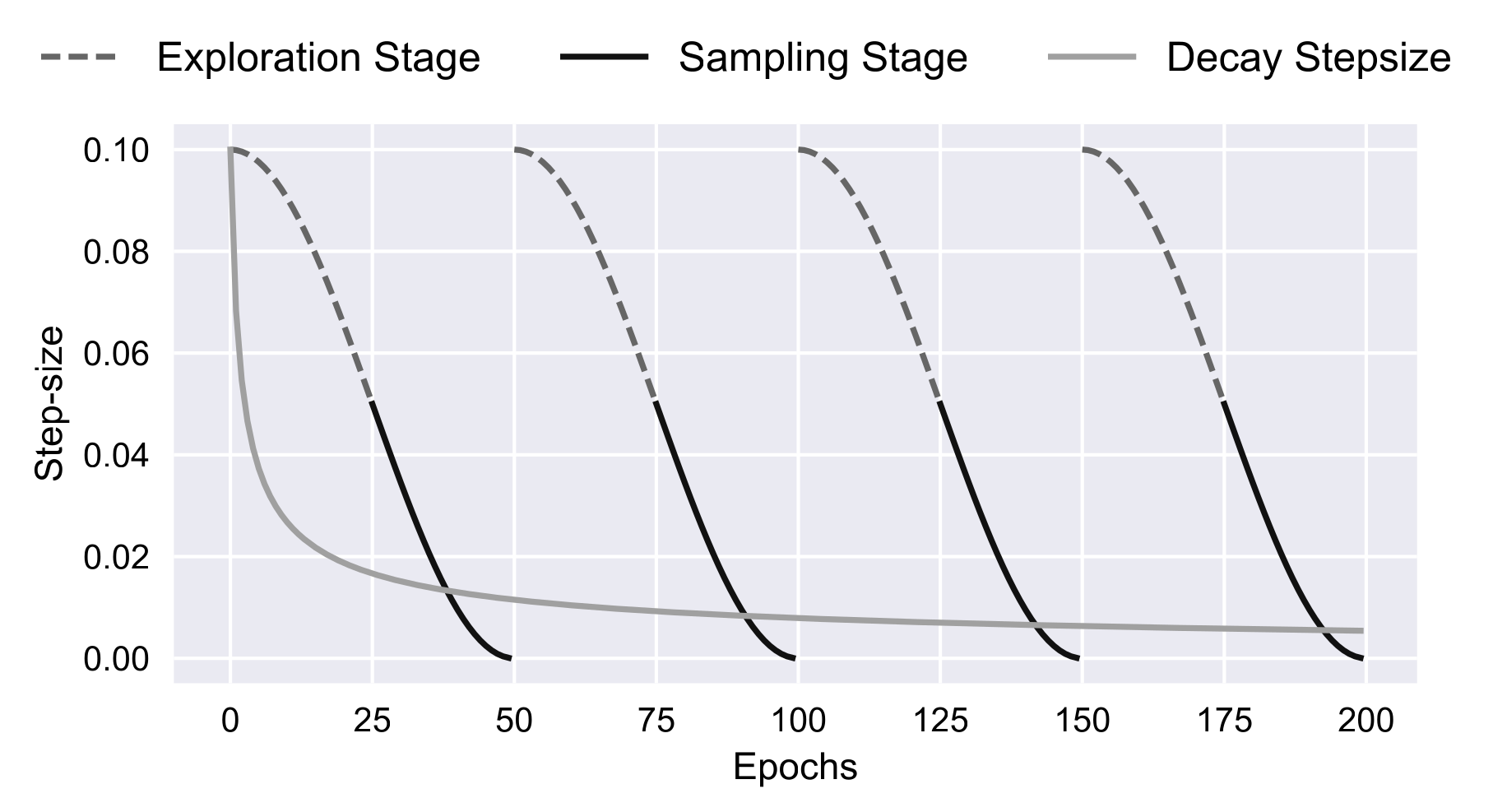
Comparison of cyclical and decaying step-size schedules. Adapted from with the permission of Ruqi Zhang. — Figure 1:Comparison of cyclical and decaying step-size schedules. Adapted from Zhang *et al.*, 2020 with the permission of Ruqi Zhang.

Sampling from Wide and Robust Local Minima¶

Distribution shift between training and test data creates a generalisation challenge for SG-MCMC algorithms Bansak et al., 2024. Local minima identified using the training data may not remain local minima under the test data, especially when they are sharp Baldassi et al., 2016Chaudhari et al., 2019. To mitigate this problem, Li & Zhang (2024) introduces Entropy-MCMC (EMCMC), which incorporates flatness-aware optimisation methods Chaudhari et al., 2019Foret et al., 2021Bisla et al., 2022 into the SG-MCMC framework. Specifically, EMCMC introduces local entropy into the posterior distribution of model parameters:

p(\widetilde{\theta}\mid\mathcal{D})=p(\theta,\theta_a\mid\mathcal{D})\propto\exp\left\{-f(\theta)-\frac{1}{2\eta}\|\theta-\theta_a\|^2\right\},

(8)

where $f(\theta)=U(\theta)$ is the negative log-posterior energy, $\eta>0$ is a coupling constant, and $\theta_a$ is an auxiliary parameter vector that locally explores the neighbourhood of $\theta$ . This posterior induces an extended energy whose gradient is

\nabla_{\widetilde{\theta}}U(\widetilde{\theta})=\left[ \begin{array}{c} \nabla_{\theta}U(\widetilde{\theta}) \\ \nabla_{\theta_a}U(\widetilde{\theta}) \end{array} \right]=\left[ \begin{array}{c} \nabla_{\theta}f(\theta)+\frac{1}{\eta}(\theta-\theta_a) \\ \frac{1}{\eta}(\theta_a-\theta) \end{array} \right].

(9)

This form provides a clear interpretation of the EMCMC sampling process: i) $\theta$ seeks low-energy regions of the energy landscape, and ii) $\theta_a$ acts as a “direction-correction force” that pulls $\theta$ away from sharp minima. Figure Figure 2 illustrates this process. EMCMC frames flatness-aware sampling as a standard MCMC process on an extended energy function without introducing an additional correction step. It also has convergence guarantees and can converge faster than previous flatness-aware methods Chaudhari et al., 2019Dziugaite & Roy, 2018.

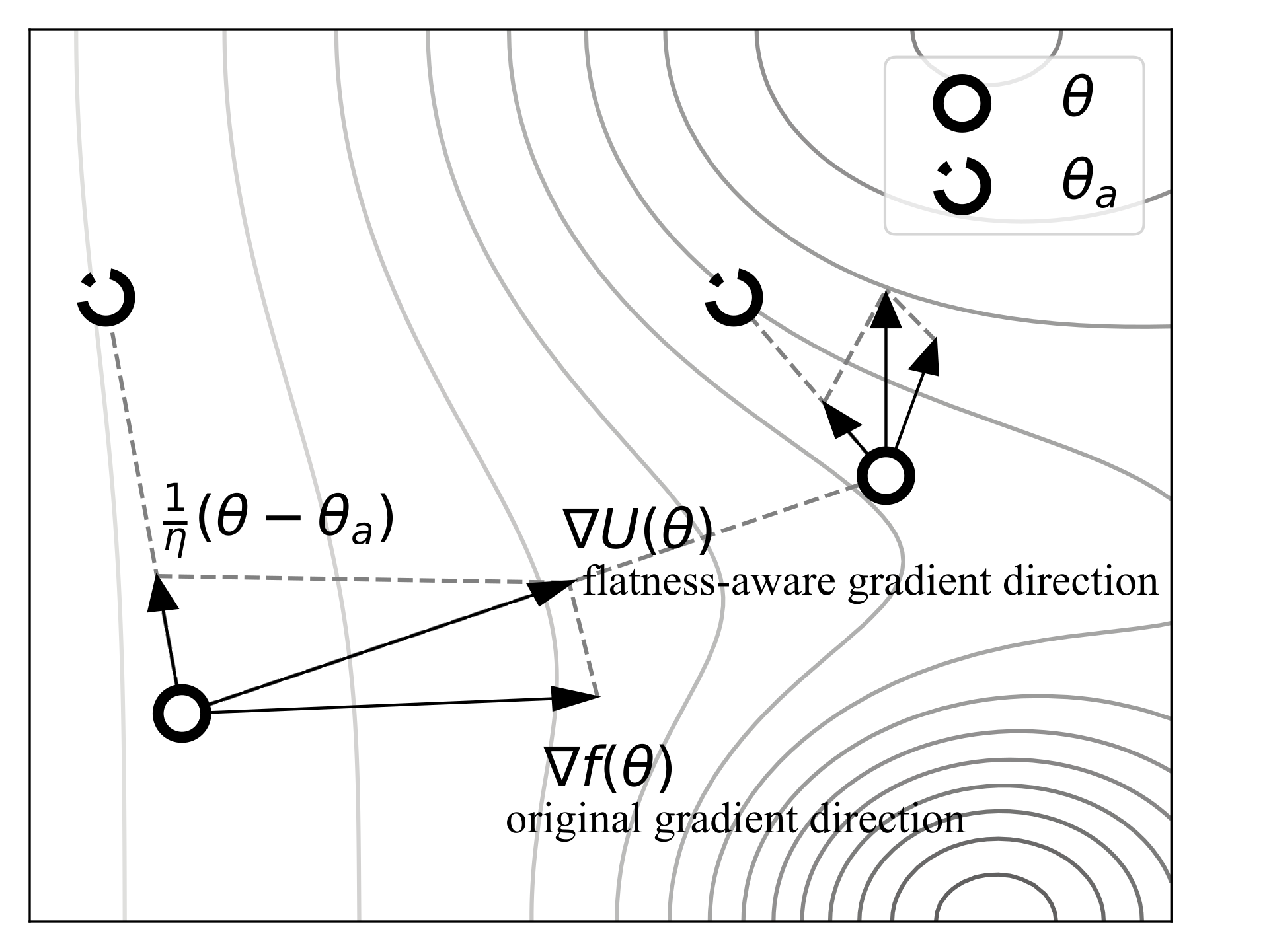
The sampling dynamics of Entropy-MCMC, showing how the guiding variable \theta_a pulls \theta toward flat regions in the energy landscape. Adapted from with the permission of Bolian Li. — Figure 2:The sampling dynamics of Entropy-MCMC, showing how the guiding variable $\theta_a$ pulls $\theta$ toward flat regions in the energy landscape. Adapted from Li & Zhang (2024) with the permission of Bolian Li.

References¶

Bottou, L. (1991). Stochastic Gradient Learning in Neural Networks. Proceedings of the International Conference on Neural Networks (Neuro-Nîmes 91).
ichi Shun-Amari. (1993). Backpropagation and stochastic gradient descent method. Neurocomputing, 5(4), 185–196.
Sebbouh, O., Gower, R. M., & Defazio, A. (2021). Almost sure convergence rates for Stochastic Gradient Descent and Stochastic Heavy Ball. In M. Belkin & S. Kpotufe (Eds.), Proceedings of Thirty Fourth Conference on Learning Theory (Vol. 134, pp. 3935–3971). PMLR.
Hastings, W. K. (1970). Monte Carlo sampling methods using Markov chains and their applications. Biometrika, 57(1), 97–109.
Chen, C., Ding, N., & Carin, L. (2015). On the Convergence of Stochastic Gradient MCMC Algorithms with High-Order Integrators. In C. Cortes, N. Lawrence, D. Lee, M. Sugiyama, & R. Garnett (Eds.), Advances in Neural Information Processing Systems (Vol. 28). Curran Associates, Inc.
Korattikara, A., Chen, Y., & Welling, M. (2014). Austerity in MCMC Land: Cutting the Metropolis-Hastings Budget. In E. P. Xing & T. Jebara (Eds.), Proceedings of the 31st International Conference on Machine Learning (Vol. 32, Issue 1, pp. 181–189). PMLR.
Quiroz, M., Kohn, R., Villani, M., & Tran, M.-N. (2019). Speeding Up MCMC by Efficient Data Subsampling. Journal of the American Statistical Association, 114(526), 831–843.
Zhang, R., Cooper, A. F., & De Sa, C. (2020). Asymptotically Optimal Exact Minibatch Metropolis-Hastings. In H. Larochelle, M. Ranzato, R. Hadsell, M. F. Balcan, & H. Lin (Eds.), Advances in Neural Information Processing Systems (Vol. 33, pp. 19500–19510). Curran Associates, Inc.
Welling, M., & Teh, Y. W. (2011). Bayesian Learning via Stochastic Gradient Langevin Dynamics. In L. Getoor & T. Scheffer (Eds.), Proceedings of the 28th International Conference on Machine Learning, ICML 2011, Bellevue, Washington, USA, June 28 - July 2, 2011 (pp. 681–688). Omnipress.
Chen, T., Fox, E., & Guestrin, C. (2014). Stochastic Gradient Hamiltonian Monte Carlo. In E. P. Xing & T. Jebara (Eds.), Proceedings of the 31st International Conference on Machine Learning (Vol. 32, Issue 2, pp. 1683–1691). PMLR.
Ding, N., Fang, Y., Babbush, R., Chen, C., Skeel, R. D., & Neven, H. (2014). Bayesian Sampling Using Stochastic Gradient Thermostats. In Z. Ghahramani, M. Welling, C. Cortes, N. Lawrence, & K. Weinberger (Eds.), Advances in Neural Information Processing Systems (Vol. 27). Curran Associates, Inc.
Jeffrey, A. (1990). Linear algebra and ordinary differential equations. Blackwell Scientific.
Chen, W., Li, B., Zhang, R., & Li, Y. (2025). Bayesian Computation in Deep Learning.
Roberts, G. O., & Tweedie, R. L. (1996). Exponential Convergence of Langevin Distributions and Their Discrete Approximations. Bernoulli, 2(4), 341–363.
Bottou, L. (1999). On-line learning and stochastic approximations. In On-Line Learning in Neural Networks (pp. 9–42). Cambridge University Press.