Simulation-based inference
Simulation-based inference (SBI) Sisson et al., 2018Cranmer et al., 2020Deistler et al., 2025 has the same goal as Bayesian inference: Given observed data and a set of beliefs, apply Bayes’ rule to update those beliefs accordingly. Unlike other Bayesian inference methods such as Markov chain Monte Carlo (MCMC) or variational inference, SBI does not rely on evaluations of the likelihood, but only on samples thereof. This makes SBI applicable to any kind of black-box function that takes in parameters and simulates observational data, a so-called forward simulator.
As an illustrative example, imagine that you are an astronomer interested in the study of planets that orbit distant stars, i.e., exoplanets. Exoplanets are usually obscured by the bright light emanating from their host stars. Astronomers observe the brightness and spectrum of these stars in a time series called a light curve, and aim to infer from these light curves properties of the exoplanets using physical models. Suppose we want to estimate the mass of an exoplanet from the light curve observations of a distant star. Using relevant physical theory, we design a computer program that maps a hypothetical mass to a simulated light curve (the “forward model”). By running such a simulator, we can obtain samples from the likelihood , but evaluating the likelihood can be computationally expensive or impossible (e.g., if the simulator takes a long time to run, or if it contains many latent variables). Simulation-based inference computes the posterior distribution while only relying on samples (or simulations) from the likelihood. To achieve this, recent SBI methods use neural networks to parameterise an “inference model” , where denotes the neural-network weights.
Introduction
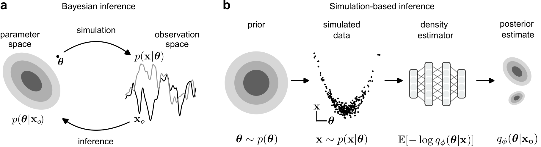
Figure 1:a: Simulators generate synthetic data (right) given parameters (left). Bayesian inference computes the posterior distribution over parameters (left) given observations (right).* b:* Simulation-based inference uses simulations (i.e., samples from the likelihood, but no likelihood evaluations) to perform Bayesian inference. A recent SBI method, Neural Posterior Estimation (NPE) uses neural networks to improve inference. NPE draws samples from the prior and runs the simulator to generate pairs of (). These data are then used to train an inference network: A conditional generative model that estimates the posterior distribution given any data . After training, the inference network is evaluated at any observation in order to draw samples from the posterior, without requiring further simulations or training. Figure modified from Deistler et al. (2025).
Classical approaches for Bayesian inference (e.g., MCMC; Chapter Introduction to sampling, or variational inference; Chapter Introduction to variational inference) rely on repeated evaluations of the likelihood and prior in order to characterise the posterior distribution and to generate samples from it. While powerful, these approaches face limitations for some forward models: Many models in science and engineering are defined as stochastic simulators, which can efficiently be run in the forward direction (i.e., their likelihood can be sampled from), but whose likelihood (as well as its gradient with respect to parameters) cannot be evaluated, or only with great computational cost Sisson et al., 2018Papamakarios, 2019Lückmann, 2021. For example, the simulator might sample a long series of latent variables before generating observations. Evaluating the likelihood of an observation would require integrating out these latent variables via
which can be computationally prohibitive even for a moderate number of latent variables. In addition, many classical Bayesian inference methods are expensive at test-time: Every time we want to perform inference on new data, we have to re-run the inference procedure, which might involve computationally expensive iterations (e.g., in MCMC sampling). As a result, it has been challenging to tackle high-throughput or real-time applications with Bayesian inference.
Simulation-based inference (SBI) methods overcome these limitations. The basic goal of SBI is to perform inference given only access to simulations (i.e., samples from the likelihood), without having to explicitly evaluate the likelihood, or any access to the internal workings of the forward model or its gradients. In addition, many SBI methods also* amortize* the cost of Bayesian inference: After an initial phase of simulation and training, they can perform inference for any new dataset within milliseconds, typically requiring only a single forward pass through a deep neural network at test time.
Early SBI methods were developed for cases in which the likelihood of the model cannot be evaluated, and are often referred to as Approximate Bayesian Computation methods Beaumont et al., 2002Marin et al., 2012Sisson et al., 2018. Wasserstein ABC provides an example of comparing observed and simulated empirical distributions directly, avoiding the need to choose summary statistics Bernton et al., 2019. More recently, the ability of SBI methods to perform inference on any black-box model, to massively parallelise model runs, and to amortize inference has expanded their scope. For example, even when the likelihood or model gradients can—in principle—be evaluated, this might require interfacing with code describing the forward model written across decades in outdated programming languages. In contrast, SBI methods entirely decouple the inference process from simulation runs, which makes it easy to apply SBI methods to simulators that are written in other programming languages or that have to be run on dedicated hardware (or, in principle, which might even correspond to a physical or living system generating the simulations from input). In other scenarios, the likelihood* can* be evaluated, but one needs fast inference for real-time or high-throughput analysis of observed phenomena, which is often out of reach for, e.g., MCMC sampling, but is possible with amortized SBI methods Dax et al., 2021. Finally, in some cases, large-scale training can also yield highly accurate and robust inference results Lueckmann et al., 2021Dax et al., 2021Deistler et al., 2022. Likely due to its simplicity, the core idea of SBI—to use forward simulations to train a supervised machine learning model—has been used in modified ways across many domains, for example, for tabular foundation models Hollmann et al., 2025.
The core insight of SBI is that performing Bayesian inference can be seen as a form of performing conditional density estimation. In recent years, a flurry of powerful conditional density estimation methods—such as normalizing flows—have been developed, often under the moniker of “Generative AI”. This has enabled an explosion of powerful new SBI methods which build on these advances, and which have been successfully applied in a wide range of scientific disciplines, e.g., in neuroscience Gonçalves et al., 2020Groschner et al., 2022Deistler et al., 2022Confavreux et al., 2023Rößler et al., 2023Hashemi et al., 2023, cognitive science Boelts et al., 2022Krause et al., 2022, biology Korfmann et al., 2023Avecilla et al., 2022, and physics Mishra-Sharma & Cranmer, 2022Dax et al., 2021Dax et al., 2025Hahn & Melchior, 2022Lemos et al., 2024Barrado et al., 2023Gebhard, Timothy D. et al., 2025Cole et al., 2022Bhardwaj et al., 2023. Here, we introduce the basic ideas and concepts of SBI. We focus on* Neural Posterior Estimation*, a conceptually simple yet powerful algorithm, but also review other approaches, diagnostic tools, and current developments. Two notable methods are* Neural Likelihood Estimation* Papamakarios et al., 2019 and* Neural Ratio Estimation* Thomas et al., 2016Hermans et al., 2020Durkan et al., 2020Miller et al., 2022, which we explain later in the chapter.
Simulation-based inference with Neural Posterior Estimation
Neural Posterior Estimation
The goal of Bayesian inference is to calculate—at least approximately—the posterior distribution of the form . Via Bayes’ rule, the posterior is proportional to the product of the prior and the likelihood , where is the normalizing constant, also called the marginal likelihood or evidence. Calculating is often challenging, and many classical Bayesian inference algorithms such as MCMC sampling therefore aim to obtain samples from the posterior without having to evaluate it. However, even these algorithms require (typically many) evaluations of the likelihood . However, many models in scientific applications are defined through numerical simulators: One can easily generate samples from the likelihood by running the simulator, but* evaluating* the likelihood can be expensive or even impossible. How can one perform Bayesian inference in such setting?
A key insight is that one does not need Bayes rule for Bayesian inference: The posterior distribution at some particular is, by definition, a conditional distribution, i.e., a normalised slice through the joint distribution at (Figure Figure 2, left). Thus, an alternative way to get the posterior is to generate a simulated dataset with—possibly many—paired samples , and then to directly estimate this posterior distribution via conditional density estimation. We can generate such a simulated dataset by first sampling the from the prior, and then, for each , to run the simulator once to get the associated , as .
We want to learn a mapping from to the distribution . One way to tackle this is to parameterise the posterior distribution by a functional form, for example, a Gaussian with mean and covariance , and to use a neural network (with parameters ) to capture the mapping from to associated posterior parameters . One can learn by maximising the log-likelihood of the parameters, i.e., by minimising the loss
where in this case, the predicted posterior probabilities would be given by a Gaussian, Blum & François, 2010Papamakarios & Murray, 2016. Thus—and provided that one can generate a large set of simulations —we have turned Bayesian inference into a supervised learning problem.
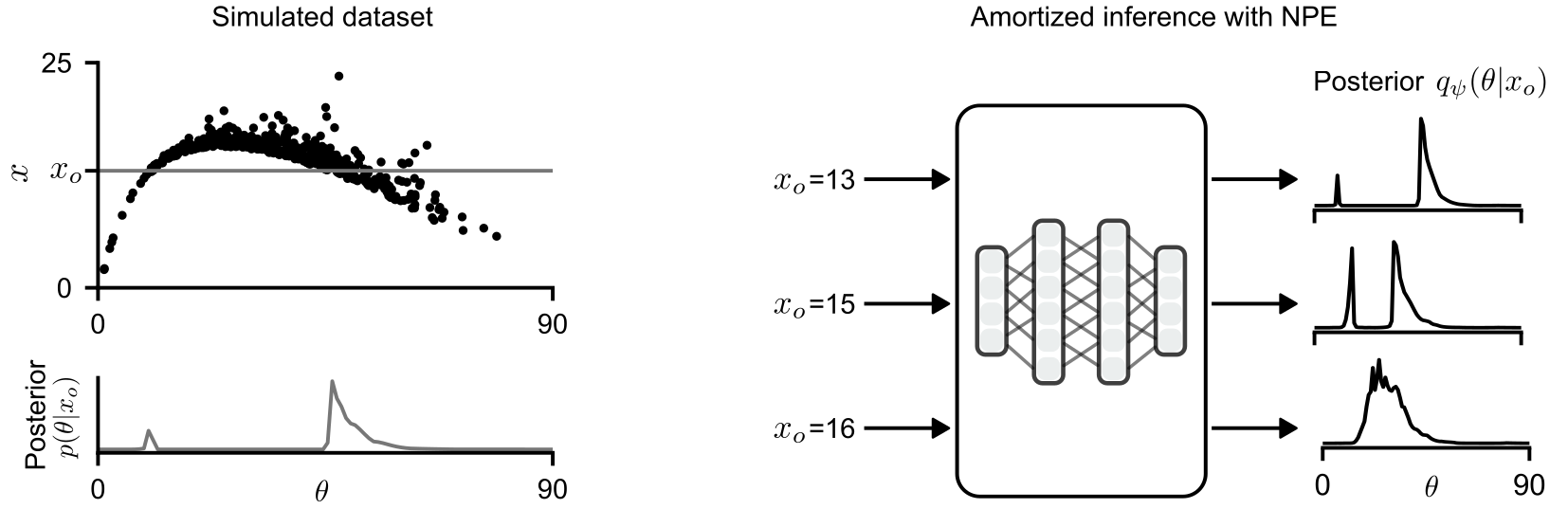
Figure 2:Framing Bayesian inference as a supervised learning problem. Left: A database of simulations (), sampled from the joint distribution by drawing samples from the prior and running the simulator. The posterior distribution (left, bottom) is a horizontal cut through the joint distribution. Right: NPE trains an inference network on these simulations. After training, the network can be evaluated at any observation and directly predicts the posterior distribution. Figure modified from Deistler et al. (2025).
Clearly, a Gaussian might be a poor approximation to the posterior, but this approach can readily be generalised to more flexible models. For example, one can use a Mixture of Gaussians Bishop, 1994Papamakarios & Murray, 2016, which requires the network to learn the mapping to multiple means , covariances and associated mixture weights . In recent years, more flexible and easy-to-train neural conditional density estimators have been proposed, which can be used for estimating non-Gaussian posteriors. In particular, Normalizing Flows Papamakarios et al., 2019 constitute a class of neural conditional densities estimators which have many favourable properties for SBI, as we will describe in the next section.
Once the conditional density estimator (sometimes referred to as inference network) has been trained on simulated data , it can readily be* evaluated* on any new observation to approximate the posterior . Indeed, it can be shown that—provided that the density estimator is sufficiently flexible, that the model is well specified, and the optimisation identifies the minimum—it will yield the true posterior Papamakarios & Murray, 2016. To demonstrate this, we rewrite the loss function (in the limit of infinite training data, i.e., in expectation of samples from ) as
The inner integral differs from the Kullback–Leibler divergence only by the conditional entropy of , which does not depend on the neural-network parameters . Therefore, if the conditional density estimator is well specified, the population loss is minimised when for -almost every .
One big advantage of these approaches is that—once the inference network has been trained—the posterior distribution for new observations can be evaluated by just plugging it into the inference network to get . Thus, inference can be performed with a single forward pass through a neural network, i.e., it is amortized (Figure Figure 2, right). Conversely, a drawback of this approach is that our simulations need to cover the entire prior, which might be wasteful as we might generate many simulations which look very different to an observation we are interested in, and which therefore do not help in constraining the relevant posterior. To address this issue (but which requires giving up on amortization), so-called* sequential* approaches have been developed, in which simulations are generated adaptively to target a posterior for a specific observation. We discuss these approaches in Section Amortized and sequential inference.
The approach described above is now commonly known as Neural Posterior Estimation (NPE). Given its conceptual simplicity and the many variations that it allows, it is challenging to track down its precise origins, and variants of it have likely been discovered independently in different application domains. Beaumont et al. (2002) and Blum & François (2010) introduced the idea of fitting a regression model from data to parameters to refine rejection-ABC approaches, which can be interpreted as NPE with a Gaussian inference network. Papamakarios & Murray (2016) showed that flexible density estimators can directly learn the posterior, when optimised with log-loss minimisation (also see Le et al. (2017)), and introduced a sequential version. Lueckmann et al. (2017) (which, to our knowledge, introduced the term (S)NPE) introduced an alternative sequential formulation, and also embedding networks for learning summary statistics from time series data. Greenberg et al. (2019) provided the first method that could use normalizing flows and is compatible with sequential learning, and used convolutional embedding nets. Ardizzone et al. (2018) proposed using invertible neural networks for solving inverse problems, resulting in an algorithm very similar to flow-based NPE, and Radev et al. (2022) popularised the amortization property of NPE.
Conditional density estimation with normalizing flows

Figure 3:Normalizing flows. Left: A target distribution which we aim to estimate based on samples. Right: Normalizing flows define a base distribution (e.g., a multivariate Gaussian) and transform this distribution through multiple transformations . After training, the transformed distribution approximates the target distribution.
As described above, a core task in SBI is to estimate the conditional distribution of parameters given some observations. Normalizing flows Papamakarios et al., 2019 have emerged as a popular conditional density estimator for SBI. They are simple and efficient to train, can be used to quickly generate samples, or to evaluate exact log-probabilities of the learned density. The latter can be useful for many downstream analyses such as maximum-a-posteriori estimation or visualisation of the posterior distribution. Finally, normalizing flows are (typically) trained by minimising the negative log-likelihood as loss function. This loss function is mass-covering, which, as we will discuss below, can be beneficial for SBI.
Normalizing flows model a target density by learning a transformation such that a random variable , which is defined to follow a simple “base” distribution (typically a multivariate standard Normal distribution) is transformed into a random variable , such that the probability density of is . The probability density modelled by such a transformation can be computed with the change of variables formula
where is the inverse of the transformation and is the determinant of the Jacobian of the inverse transformation . Normalizing flows stack many transformations in order to model complicated densities.
To evaluate Equation (4) and to efficiently train normalizing flows, the transformation must be a diffeomorphism (i.e., it must be differentiable and invertible). In addition, the Jacobian of is of size (for densities of dimensionality ), and computing the determinant of such a matrix is typically of computational complexity , which would be prohibitive for large . As such, normalizing flows require that the transformation is constructed such that the determinant of the Jacobian can be evaluated efficiently. Normalizing flows differ in how they define the transformation such that it fulfills these criteria. A popular class of transformations are autoregressive flows, and within SBI, masked autoregressive flows Papamakarios et al., 2017 and neural spline flows Durkan et al., 2019 are particularly popular. These normalizing flows define bijective transformations for every individual dimension and then couple dimensions with neural networks.
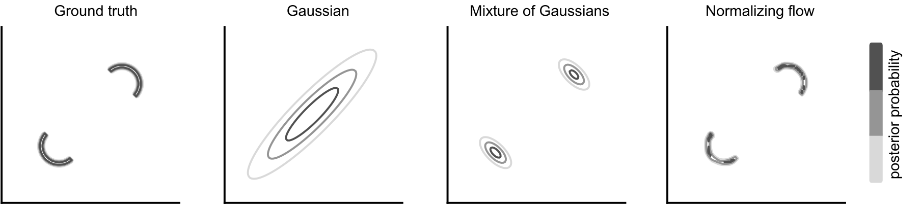
Figure 4:Expressiveness of different generative models for approximating the posterior distribution with NPE. The ground truth posterior (left) consists of two moons and has low posterior density in between. Using a Gaussian (second from left) as generative model produces a poor—albeit mass-covering—posterior distribution. A mixture of multiple Gaussians (second from right) improves accuracy, but fails to produce the moon shapes. Normalizing flows (right) enable NPE to accurately capture complex posterior distributions.
Normalizing flows train the transformations by minimising the negative log-likelihood of the data
In neural posterior estimation (NPE), normalizing flows are used to estimate the posterior probability density . To estimate a conditional probability density, NPE conditions that transformation on data , or an embedding thereof (Section Learning from high-dimensional data with embedding networks). This enables NPE to learn different posterior distributions for different data.
The normalizing flow is then trained over pairs of parameters and simulation outputs, where the parameters are sampled from the prior. NPE minimises the loss
If the normalizing flow is well-specified, i.e., the true conditional posterior belongs to the family of normalizing-flow models, then there exists some such that for -almost every , where denotes the parameter space. In this case, the population loss is minimised at the true conditional posterior, assuming successful optimisation. After training, one can then sample from the posterior for any observation by drawing a sample from the base distribution and transforming it with the series of transformations (which are conditioned on ). Notably, samples from normalizing flows are i.i.d. and follow the estimated density exactly (i.e., normalizing flows do not require any approximations to draw samples from the modelled density). In addition, normalizing flows can also evaluate the density of parameters under the posterior via Equation (4).
An important property of this loss is that it tends to be mass-covering: it will strongly penalise the normalizing flow being too narrow (as becomes a large negative number, leading to very high loss). As such, for limited training data or for imperfect convergence of the normalizing flow, will tend towards being broader than the true posterior distribution . In many applications of SBI, this is a desirable feature: too narrow posteriors would indicate overly confident parameter estimates, which could lead to wrong claims of scientific discovery Hermans et al., 2022. This mass-covering behaviour is in contrast to variational inference, which typically uses divergence objectives whose covering or seeking behaviour depends on the divergence direction, with common formulations tending to be mode-seeking (i.e., towards a too narrow posterior approximation) Li & Turner, 2016. Since we operate with finite samples, none of these are guarantees.
Learning from high-dimensional data with embedding networks
Many models in science and engineering produce high-dimensional simulation outputs such as images or long time series. In order to estimate parameters underlying such data, NPE can be combined with embedding networks (Figure Figure 5) Lueckmann et al., 2017. Embedding networks are neural networks which take as input high-dimensional data and return a lower-dimensional summary statistic of them. These summary statistics are then passed to the inference network, which uses the summary statistics to approximate the posterior. Ideally, these summary statistics will be (approximately) sufficient, i.e., still preserve all relevant information for the posterior, so that Fearnhead & Prangle, 2010Chen et al., 2020.
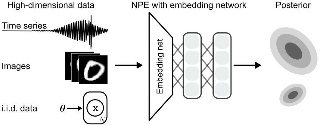
Figure 5:Neural Posterior Estimation (NPE) with embedding networks. Left: For many models, simulation outputs can be high-dimensional. For example, simulators might produce long time series, images, or i.i.d. data given a particular parameter set. Middle: In order to perform inference based on such observations, NPE can be combined with suitable embedding networks that efficiently reduce these data to lower-dimensional summary statistics. These summary statistics are then processed by the inference network, and both neural networks can be trained end-to-end. Right: Illustration of a posterior distribution underlying such observations.
In NPE, the embedding network can be trained end-to-end with the inference network, that is, with the log-likelihood loss specified in Equation (6). Provided that the embedding network is sufficiently expressive, it will automatically learn appropriate summary statistics, without requiring separate data-compression methods Chen et al., 2020 (although those might still be empirically useful in some cases Chen et al., 2023). The choice of embedding network depends on the type of data modelled by the simulator. For example, for images, a popular choice for the embedding net are convolutional neural networks (CNNs), and recurrent neural networks (RNNs) might be useful for time-series data Lueckmann et al., 2017.
An important case is the setting in which the observation does not constitute a single observation, but rather stands for a set of observations which are thought to be sampled i.i.d. from the same parameter. In this case, the posterior distribution should be invariant to the ordering of the observations, which can be achieved by using a permutation invariant embedding network such as a set transformer Lee et al., 2019, as proposed by Chan et al. (2018) for applications in population genetics. Radev et al. (2022) proposed and evaluated using such networks for datasets with varying size.
Instead of learning summary statistics end-to-end with an embedding network, one can also manually extract summary statistics from the data and perform inference based on these statistics. This requires domain knowledge and, if the choice of summary statistics is poor, might lead to a significant loss of information about parameters, but it can be beneficial if one is interested in inferring parameters given particular features of data. Indeed, in many cases, the simulator is not able to reproduce all features of the (experimentally) observed data. Manually defined summary statistics can avoid such misspecification by focusing only on properties of the data which can be modelled by the simulator.
Amortized and sequential inference
As described above, NPE amortizes the cost of inference: After training on a simulated dataset generated from prior predictives (i.e., simulation results based on parameters drawn from the prior distribution), they can perform inference for* any* new observed data . In cases where one is interested in performing inference for many different observations, or where inference is time-critical, this can be highly beneficial. In cases where one only aims to perform inference for a single observation (or for few observations), NPE can be wasteful: By training a neural network on* prior* predictives, the neural network has to learn from a broad range of (simulated) data, even though it is eventually only evaluated at few observations.
Sequential methods have been developed to improve the simulation-efficiency of SBI in these cases. These methods draw parameters (which are then used to generate the training dataset) from a “proposal” distribution. This proposal distribution is chosen such that simulation outputs are expected to be closer to the observation than prior predictives. A popular choice for the proposal distribution is the posterior distribution obtained by running NPE with a limited number of simulations (but explicit active learning schemes have also been proposed Griesemer et al., 2024).
These methods are often called sequential, as the inference network is trained across multiple, sequentially simulated datasets, where the approximate posterior after each round guides generation of the next dataset. It has been demonstrated that sequential methods can improve simulation efficiency, often by an order of magnitude or more Lueckmann et al., 2021Glöckler et al., 2022Deistler et al., 2022. While potentially reducing the number of required simulations, using sequential methods with NPE can have a drawback: Drawing parameters from a proposal distribution (instead of from the prior) biases the posterior distribution towards regions that were oversampled in the proposal (compared to the prior). Several methods have been developed to overcome this. Papamakarios & Murray (2016) proposed to train the neural network with the standard log-likelihood loss, and to then correct the posterior post-hoc. Lueckmann et al. (2017) suggested to importance-weight the loss, such that the density estimator directly approximates the posterior after training. Greenberg et al. (2019) introduced a contrastive loss, which implicitly frames conditional density estimation as a classification problem Durkan et al., 2020, and which can be combined with arbitrary acquisition functions Griesemer et al., 2024. Finally, Blum & François (2010) and Deistler et al. (2022) proposed to draw parameter sets from a restricted region of the prior, such that no modifications of the loss function or post-hoc corrections are required. Notably, for many other SBI methods, such as Neural Likelihood Estimation, NLE Papamakarios et al., 2019Lueckmann et al., 2018, or Neural Ratio Estimation, NRE Hermans et al., 2020Thomas et al., 2016Durkan et al., 2020Miller et al., 2022, parameters for the training dataset can be drawn from* any* distribution and the neural networks can nonetheless be trained with standard loss functions, as the prior is explicitly taken into account during inference with MCMC or variational inference.
Evaluating the correctness of SBI methods
The problem of evaluating SBI methods
After having obtained an approximate posterior with SBI methods, a central challenge is to evaluate the quality of this posterior. This is difficult because, for any real-world task, the ground-truth posterior is unavailable.
Several diagnostic tools have been developed to overcome this limitation. Note, however, that many of these tools do not provide sufficient conditions for posterior correctness. Instead, they provide* necessary* conditions for posterior correctness, and thus enable detection of inaccuracies in the posterior estimate. Other methods can, in principle, provide sufficient conditions for correctness, but rely on additional hyperparameters or the accuracy of other trained neural networks, which can compromise the accuracy of the diagnostic tool. Below, we focus on a set of diagnostic tools called coverage diagnostics, and we then briefly describe other methods.
Coverage diagnostics
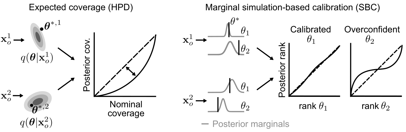
Figure 6:Coverage diagnostics for identifying inaccuracies in the approximate posterior. Left: Expected coverage based on the highest-probability density (HPD) region aims to detect whether the joint posterior distribution is over- or under-confident. Marginal simulation-based calibration (SBC) aims to detect inaccuracies in the marginals of the posterior distribution. Both of these methods produce rank distributions, which are optimal if the posterior lies on the diagonal, and indicate issues if it lies above or below the diagonal. Figure modified from Deistler et al. (2025).
A set of diagnostic tools that aim to detect inconsistencies in the posterior distribution are coverage diagnostics Cook et al., 2006Talts et al., 2018. These methods begin by generating a calibration dataset: They sample parameters from the prior and run the simulator to generate samples . For every in the calibration dataset, these methods then draw samples from the posterior obtained with an SBI method. For amortized SBI methods, this process is fast, as inference can be performed for any without retraining or resimulating.
Coverage diagnostics then reduce posterior samples and the ground truth parameters to 1-dimensional quantities, via a reducing function , where is the parameter dimensionality. The posterior approximation is calibrated if, for any reducing function , the rank of is distributed uniformly within (Figure Figure 6). Different diagnostic tools use different mappings to detect posterior inconsistencies. For example, can compute the posterior log-probability (often referred to as* expected coverage* based on the highest-probability density (HPD) region) Miller et al., 2021Hermans et al., 2022Deistler et al., 2022, or it can pick the 1D marginals of Cook et al., 2006Talts et al., 2018. In the former case, coverage diagnostics can detect inconsistencies in higher-order moments of the posterior (Figure Figure 6, left). In the latter case, coverage diagnostics cannot detect inconsistencies in higher-order moments of the posterior, but they can provide intuition about which parameter is inconsistent (Figure Figure 6, right).
A core advantage of coverage diagnostics is that they can be run with relatively small calibration sets (typically, simulations), and that they do not require further tuning of hyperparameters or training of a “diagnostic neural network”. This makes them robust and easy to deploy. However, coverage diagnostics typically provide a necessary, but not a sufficient condition for posterior correctness. In particular, if the approximate posterior always returns the prior distribution (instead of an approximation to the posterior), then it passes the above described coverage diagnostics. This highlights the need for additional diagnostic tools.
Other methods
A simple tool for diagnosing the posterior approximation is to perform Posterior Predictive Checks (PPCs). Given an observation, these methods draw samples from , simulate them, and then compare the simulation outputs (the posterior predictives) to the observation. For every posterior sample , it should be possible to obtain a simulation result that closely matches the observation. If posterior predictive checks fail (e.g., because all posterior predictives are far away from the observation, or if some parameter sets can* never* match the observation), then this indicates issues in the accuracy of . In particular it might be trained on too few simulations, or it might hint towards* model misspecification* (a case where the observation cannot be matched by* any* parameter set, as discussed in Section Current developments).
Beyond coverage checks and PPCs, many other diagnostic tools for SBI have been developed over the past years. For example, some local calibration diagnostics aim to provide sufficient and necessary conditions for posterior correctness Linhart et al., 2023Säilynoja et al., 2025. However, these methods often require to train an additional neural network and hinge on the accuracy of that additional trained neural network. Because of this, these diagnostic tools require larger calibration datasets and might themselves have issues (e.g., due to poor convergence of the additional trained neural network).
Alternative methods
Neural Posterior Estimation (NPE) directly estimates the posterior distribution. In addition to NPE, researchers have developed other methods for SBI. These approaches train neural networks to emulate either the likelihood (Neural Likelihood Estimation, NLE) or the likelihood-to-evidence ratio (Neural Ratio Estimation, NRE) and then use traditional Bayesian inference methods (e.g., MCMC) to draw samples from the posterior. Finally, some recent methods also go beyond estimating only the posterior or the likelihood(-ratio). Below, we describe these alternative methods for SBI.
Likelihood estimation
Neural Likelihood Estimation (NLE) uses neural density estimators (such as conditional normalizing flows) to estimate the likelihood Papamakarios et al., 2019. This estimate can be learned from samples of the joint distribution by optimising the negative log likelihood of simulation outputs given parameters. NLE trains a conditional density estimator , such as a normalizing flow, by optimising towards the objective
After training, the trained model can be used to emulate the simulation process by drawing samples from the likelihood approximation .
For posterior inference, the trained model is multiplied by the prior to obtain the (unnormalised) posterior estimate
In order to draw samples from the (approximate) posterior distribution , a method to draw samples from an unnormalised distribution is necessary, for example, rejection sampling or Markov chain Monte Carlo (Section Sampling from the approximate posterior using unnormalised inference models). Normalizing flows enable (differentiable) evaluation of the likelihood approximation , making this possible, albeit being potentially computationally expensive. Variational inference has been shown to speed up high-dimensional sampling from NLE Wiqvist et al., 2021Glöckler et al., 2022. However, any of these sampling methods are typically slow and can introduce additional errors into the inference procedure. An additional disadvantage of NLE (compared to NPE) is that it cannot be combined with an embedding network that is trained end-to-end. One can embed before training with a separate neural network, e.g., an autoencoder, then perform NLE on the embedded simulation outputs Chen et al., 2020.
NLE can also be used in a sequential scheme to reduce the number of required simulations for inference given a particular observation. These sequential NLE methods focus on a specific observation , generating data nearby iteratively Papamakarios et al., 2019. A major advantage of NLE in that scenario is that it does not require modifications of the loss function: The neural density estimator will converge to the likelihood for any distribution from which parameters are drawn.
Likelihood-to-evidence ratio estimation
The likelihood-to-evidence ratio is a natural estimation target for simulation-based inference because Bayes’ rule gives . Ratio estimators allow more flexible architectures than diffeomorphic normalizing flow layers with tractable determinants. However, density ratios can span many orders of magnitude and therefore be numerically difficult to approximate directly. For this reason, one typically estimates . A stable approach to estimating converts the problem into a classification task. Several variants have been developed Cranmer et al., 2015Durkan et al., 2020Miller et al., 2022Thomas et al., 2016; here, we focus on the method of Hermans et al. (2020).
NRE introduces a binary class label and defines the joint distribution . We assign equal class probabilities, , and define the class-conditional distributions as
is called the product of marginals. It is best understood algorithmically: One takes two independent samples and simulates one of them . Then the samples are distributed . Sampling from the joint is achieved by first sampling the prior and simulating . We then have a sample .
Bayes’ rule shows why this classification problem identifies the desired ratio:
Consequently, , where denotes the sigmoid function. We therefore construct
where is a classifier, with , and is a likelihood-to-evidence ratio estimate. Both are parameterised by the neural network with weights . We optimise by minimising the conditional KL divergence,
Here, is the marginal mixture induced by the constructed classification problem:
The conditional KL divergence differs from the binary cross-entropy used to train the classifier only by the conditional entropy of , which is constant with respect to . The two objectives therefore have the same minimiser. Assuming sufficient model capacity and successful optimisation, the conditional KL divergence is zero at the optimum, so and almost everywhere under .
We can now form the unnormalised posterior approximation . Unless the classifier recovers the exact ratio, need not integrate to one. Its normalised counterpart is
with . At the exact optimum, and hence . In practice, posterior behaviour is usually characterised using samples, and samplers for unnormalised distributions do not require to be computed.
One can draw samples from using any sampling method for unnormalised distributions, just like with NLE (Section Sampling from the approximate posterior using unnormalised inference models). The ratio-based neural network can be both more expressive and cheaper than the normalizing flow-based likelihood approximation from NLE. Flows require parameterising an efficient diffeomorphism with a tractable log determinant, whereas NRE permits arbitrary neural-network architectures. One limitation is that the standard NRE objective in (12) does not generally attain the same asymptotic efficiency as maximum-likelihood density estimation Rhodes et al., 2020Choi et al., 2022Yu et al., 2025. Alternative objectives have therefore been explored for ratio estimation Glaser et al., 2022Miller et al., 2023.
Sampling from the approximate posterior using unnormalised inference models
While NPE approximates the posterior directly, NLE and NRE require an additional inference step to draw samples from the posterior. To this end, one can use general-purpose sampling methods (see Chapter Introduction to sampling) and adapt them to sample from an unnormalised posterior estimate. Rejection sampling or reweighted sampling from the prior are natural choices for simple problems with low dimensionality due to straightforward embarrassingly parallel implementations Murphy, 2012. Both of these methods start by drawing samples from the prior
In rejection sampling, we choose a constant such that for all in the support of , where denotes the unnormalised posterior density. For each of the samples, we draw
where we let denote the one-dimensional uniform distribution between and . This algorithm yields samples from the approximate posterior in the following way:
Rejection sampling generates samples, on average. It is efficient when , i.e., in low dimensions and when the prior and approximate posterior have similar support. Rejection sampling is inefficient when the approximate posterior is narrow compared to the prior.
In reweighted sampling, we use the samples from the prior in (15), but assign them a self-normalised importance weight. The weights and self-normalised weights are defined as
Histograms and moments of the distribution can be computed using weighted samples . The variance of the weights can be large, implying one sample takes most of the probability mass. This occurs in the same situations when rejection sampling is inefficient.
One sampling method that can be more robust to high dimensionality and approximate posteriors that make up only a small volume (compared to the prior) is Markov chain Monte Carlo. Rather than explaining further, we simply define the Metropolis-Hastings acceptance probability and refer the reader to Chapter Introduction to sampling. Given a fixed and proposal distribution with transition density from to , the acceptance probability in a Metropolis-Hastings step is
This acceptance probability does not depend on and can therefore draw samples from the approximate posterior even when is not normalised. Designing an efficient transition kernel and identifying convergence is an open area of research.
Estimating multiple quantities at once
Finally, some recent methods go beyond estimating the posterior, the likelihood, or the likelihood-ratio and estimate several of these quantities, typically with separate models Wiqvist et al., 2021Glöckler et al., 2022Radev et al., 2023. Recently, the Simformer Gloeckler et al., 2024 has been proposed to estimate the full joint distribution as well as all of its conditionals and marginals in a single model, based on transformers and a diffusion model. Thereby, the Simformer improves the flexibility of SBI and it combines desirable features of NPE (e.g., to directly draw samples from the posterior) and NLE (e.g., to emulate the simulator).
Current developments
Neural Posterior Estimation (NPE), as well as alternative methods such as Neural Likelihood Estimation (NLE) or Neural Ratio Estimation (NRE), have been demonstrated as powerful tools for SBI. Over the past years, researchers have extended these methods in many ways, and have developed new SBI methods that go beyond estimating the posterior or likelihood(-ratio). We outline recent trends in using neural networks for SBI.
Better generative models
Normalizing flows have been a popular choice for NPE for several years, likely due to their robustness in training, their ability to quickly (and exactly) evaluate the log-probability of samples, and their mass-covering property. However, the fact that the transformation trained by normalizing flows has to be invertible can constrain the flexibility of the normalizing flow. This may reduce the accuracy of posterior estimates of normalizing flows, especially for high-dimensional and structured parameter spaces (e.g., if the parameters are a time series or an image). To overcome this, recent methods have explored other conditional generative models for NPE. In recent years, diffusion models have been particularly popular due to their ability to estimate high-dimensional parameter spaces, and to maintain the ability to evaluate the log-probability via the probability flow ODE (albeit at significantly higher computational cost) Sharrock et al., 2022Geffner et al., 2023Gloeckler et al., 2024. Many other generative models have been explored for NPE, ranging from flow-matching Wildberger et al., 2023 to consistency models Schmitt et al., 2024, generative adversarial networks Ramesh et al., 2022, energy-based models Glaser et al., 2022, and tabular foundation models Vetter et al., 2025. We expect that any major advances in (conditional) generative modelling will directly carry over to improvements in NPE.
Improving the flexibility of simulation-based inference
A core limitation of NPE with normalizing flows is that it requires the inference task to be known upfront. If, for example, the prior changes, when the simulator is modified, or when the data representation changes, NPE has to be re-run in order to perform inference (including running simulations and training the neural network).
To overcome this, many recent methods have improved the flexibility of NPE. First, in order to perform inference given any number of i.i.d. trials, permutation-invariant embedding networks can be used, as described above Radev et al., 2022. Alternatively, diffusion models enable NPE to estimate the posterior distribution given any number of i.i.d. datapoints, even when the neural network was trained on pairs of parameters and a single simulation result Geffner et al., 2023Linhart et al., 2026Gloeckler et al., 2024. Second, in order to enable more flexible specification of prior or simulator, it has been proposed to amortize over hyperparameters of prior or simulator Starostin et al., 2025Elsemüller et al., 2023Müller et al., 2023. In that case, the inference network is conditioned not only on data, but also on additional values describing the prior or simulator. At inference time, one can then perform inference for any prior and for any simulator. Third, in some cases and only for some observations, some parameters may be known and should not be inferred, but instead should be kept fixed Deistler et al., 2022Gloeckler et al., 2024. In other cases, data may not always be complete, and parts of an observation might be missing. In order to flexibly perform amortized inference in these cases, several methods enable the estimation of any parameter conditional of NPE and systematically deal with missing data Rozet & Louppe, 2021Deistler et al., 2022Gloeckler et al., 2024Verma et al., 2025.
Improving robustness to model misspecification
A fundamental challenge for SBI emerges when the simulator is misspecified, i.e., when it does not match reality. In the most extreme case, the observation cannot be generated by the simulator (i.e., the combination of prior and simulator) with any set of parameters and with any level of simulator noise.
This can have a drastic impact on SBI: While one might expect that, for misspecified observations, the approximate posterior will have mass in parameter regions that generate predictives that are close to the observation, or that the approximate posterior should be very uncertain, this is not the case. Indeed, neural network-based methods for SBI have been shown to react erratically to the misspecified observations and can produce non-sensible posteriors Cannon et al., 2022.
Several methods have been proposed to improve the robustness of SBI in these scenarios, including adding noise to the simulation outputs Ward et al., 2022, learning statistics of the observations Huang et al., 2023 such that they are not misspecified, training on unlabelled Mishra et al., 2025 and labelled Wehenkel et al., 2024 observations when available, or changing the target of inference Gao et al., 2023.
Conservative and calibrated posterior approximations
Approximate SBI posteriors can be overconfident[1], particularly when simulations are limited, motivating methods that promote conservative or calibrated uncertainty estimates Hermans et al., 2022. Balanced neural ratio estimation modifies the NRE training objective to favour conservative approximations, while preserving its Bayes-optimal solution Delaunoy et al., 2022, by effectively regularising the estimate to be closer to the prior. This balancing principle has also been extended to NPE and contrastive NRE Delaunoy et al., 2023. Alternatively, differentiable relaxations of coverage error can be included directly in the training objectives of amortized SBI methods, encouraging calibrated posteriors with moderate additional computational cost Falkiewicz et al., 2023. However, expected coverage is a necessary rather than sufficient diagnostic: an approximation can exhibit nominal coverage while still differing substantially from the true posterior. Ratio coverage plots address some of these blind spots by comparing the approximate and true posteriors through an estimated density ratio Lipp et al., 2026.
Discussion
Many processes in the natural sciences and in engineering are best described by complex, stochastic, and potentially non-differentiable simulators. For many such models, the likelihood can become excessively expensive or even impossible to evaluate. In order to perform inference with traditional Bayesian inference methods such as MCMC, scientists and engineers had to modify their model such that the likelihood can be efficiently evaluated, but which comes at the cost of reducing the fidelity of the simulator.
Simulation-based inference (SBI) makes Bayesian inference accessible to the widest class of models: It can be applied to any black-box simulator for which one can run forward simulations. In recent years, neural networks have largely improved the accuracy and applicability of SBI. These methods generate a database of parameters and corresponding simulation outputs, and then train neural networks to learn the statistical relationship between these quantities. After training, the neural network can be evaluated at any observation and enables us to infer the posterior distribution without further simulations or retraining.
SBI with neural networks has already been applied to perform inference in a wide range of disciplines in science and engineering. We expect that the continued progress in improving the accuracy, flexibility, and robustness of these approaches will have a profound impact on many fields, and we hope that it will enable new scientific discoveries.
This occurs when the approximate posterior is narrower than the ground truth.
- Sisson, S. A., Fan, Y., & Beaumont, M. A. (2018). Overview of Approximate Bayesian Computation.
- Cranmer, K., Brehmer, J., & Gilles Louppe. (2020). The frontier of simulation-based inference. Proceedings of the National Academy of Sciences, 117(48), 30055–30062.
- Deistler, M., Boelts, J., Steinbach, P., Moss, G., Moreau, T., Gloeckler, M., Rodrigues, P. L. C., Linhart, J., Lappalainen, J. K., Miller, B. K., Gonçalves, P. J., Lueckmann, J.-M., Schröder, C., & Macke, J. H. (2025). Simulation-Based Inference: A Practical Guide.
- Papamakarios, G. (2019). Neural Density Estimation and Likelihood-free Inference.
- Lückmann, J.-M. (2021). Simulation-based inference for neuroscience and beyond [Phdthesis]. Dissertation, Tübingen, Universität Tübingen, 2022.
- Beaumont, M. A., Zhang, W., & Balding, D. J. (2002). Approximate Bayesian computation in population genetics. Genetics, 162(4), 2025–2035.
- Marin, J.-M., Pudlo, P., Robert, C. P., & Ryder, R. J. (2012). Approximate Bayesian computational methods. Statistics and Computing, 22(6), 1167–1180.
- Bernton, E., Jacob, P. E., Gerber, M., & Robert, C. P. (2019). Approximate Bayesian computation with the Wasserstein distance. Journal of the Royal Statistical Society: Series B (Statistical Methodology), 81(2), 235–269.
- Dax, M., Green, S. R., Gair, J., Macke, J. H., Buonanno, A., & Schölkopf, B. (2021). Real-Time Gravitational Wave Science with Neural Posterior Estimation. Phys. Rev. Lett., 127(24), 241103.
- Lueckmann, J.-M., Boelts, J., Greenberg, D., Goncalves, P., & Macke, J. (2021). Benchmarking Simulation-Based Inference. In A. Banerjee & K. Fukumizu (Eds.), Proceedings of The 24th International Conference on Artificial Intelligence and Statistics (Vol. 130, pp. 343–351). PMLR.
- Deistler, M., Macke, J. H., & Pedro J. Gonçalves. (2022). Energy-efficient network activity from disparate circuit parameters. Proceedings of the National Academy of Sciences, 119(44), e2207632119.
- Hollmann, N., Müller, S., Purucker, L., Krishnakumar, A., Körfer, M., Hoo, S. B., Schirrmeister, R. T., & Hutter, F. (2025). Accurate predictions on small data with a tabular foundation model. Nature, 637(8045), 319–326.
- Gonçalves, P. J., Lueckmann, J.-M., Deistler, M., Nonnenmacher, M., Öcal, K., Bassetto, G., Chintaluri, C., Podlaski, W. F., Haddad, S. A., Vogels, T. P., Greenberg, D. S., & Macke, J. H. (2020). Training deep neural density estimators to identify mechanistic models of neural dynamics. eLife, 9, e56261.
- Groschner, L. N., Malis, J. G., Zuidinga, B., & Borst, A. (2022). A biophysical account of multiplication by a single neuron. Nature, 603(7899), 119–123.
- Confavreux, B., Ramesh, P., Goncalves, P. J., Macke, J. H., & Vogels, T. (2023). Meta-learning families of plasticity rules in recurrent spiking networks using simulation-based inference. In A. Oh, T. Naumann, A. Globerson, K. Saenko, M. Hardt, & S. Levine (Eds.), Advances in Neural Information Processing Systems (Vol. 36, pp. 13545–13558). Curran Associates, Inc.