Sequential Monte Carlo samplers
This chapter develops sequential Monte Carlo (SMC) samplers as a population-based approach to inference in Bayesian deep learning.[1] Building on the sequential Monte Carlo methods of Chapter Introduction to sampling, we focus on the two extensions that make them practical for neural network posteriors: multilevel SMC and scalable parallel SMC.
Motivation
Chapter Introduction to sampling introduced SMC as a particle filter Doucet et al., 2001Doucet & Johansen, 2011: a latent state evolving in time, tracked by a population of particles over a sequence of growing spaces. This chapter applies the same population-based approximation to a static target—a Bayesian posterior on a fixed parameter space. Without any dynamics to generate them, the intermediate distributions are now constructed by design, and the resulting methods are known as SMC samplers Del Moral et al., 2006.
It is useful to place the neighbouring methods relative to this sampler. Tempering is the mechanism inside the sampler that builds the intermediate distributions, annealing the likelihood from the prior to the posterior Geyer, 1991Gelman & Meng, 1998Neal, 2001 (data-tempering Chopin, 2002 is a common alternative). Annealed importance sampling (AIS) is the reduced case in which resampling is omitted Neal, 2001, so it is best viewed as a simplified SMC sampler rather than a distinct method. The chapter’s two main contributions are developments of the SMC sampler, along two different axes: multilevel SMC (MLSMC) improves statistical efficiency by combining a hierarchy of coarse-to-fine approximations in a telescoping estimator Beskos et al., 2017Beskos et al., 2018, while parallel SMC improves scalability by running many samplers concurrently and weighting them by their normalizing-constant estimates, avoiding the heavy communication of island particle methods Vergé et al., 2015Whiteley et al., 2016Liang et al., 2025.
These methods matter for Bayesian deep learning because neural network posteriors are high-dimensional, multi-modal with many symmetric modes, and costly to evaluate—the regime where importance sampling degenerates and single-chain MCMC mixes slowly. An SMC sampler anneals an entire population towards the posterior, provides an unbiased estimate of the model evidence, and parallelises naturally. The remainder of the chapter develops the two extensions that make this practical at scale: MLSMC with trace-class neural network priors Sell & Singh, 2023Chada et al., 2025, and scalable parallel SMC Liang et al., 2025.
Introduction
Monte Carlo based Bayesian algorithms of the type described in Chapter Introduction to sampling typically require generating many samples from a target distribution which at best can be evaluated up to a normalizing constant. This can be expensive and cumbersome in high-dimensions, and so methods to improve complexity are paramount. As discussed in Chapter Introduction to sampling, the best computational complexity achievable by a Monte Carlo algorithm in general is cost MSE, i.e. achieving a mean square error (MSE) of for will asymptotically require samples. This is hence referred to as the canonical rate, as it holds for any intractable integral for which we can generate i.i.d. unbiased samples of the integrand.
The sequential Monte Carlo (SMC) sampler Del Moral et al., 2006Dai et al., 2022Chopin & Papaspiliopoulos, 2020 was developed at the turn of the millennium Jarzynski, 1997Berzuini & Gilks, 2001Gilks & Berzuini, 2001Neal, 2001Chopin, 2002, and is well suited to this high-dimensional regime. Forcing the (successive) importance distributions to be close provides a generic mechanism to overcome the “curse-of-dimensionality”, i.e. complexity* constant* scaling like for dimension Chatterjee & Diaconis, 2018Agapiou et al., 2017. Under suitable high-dimensional stability assumptions, SMC samplers can avoid the exponential degradation of direct importance sampling and may achieve polynomial cost scaling in dimension Beskos et al., 2014. The SMC sampler also handles bad initialization or multi-modality on par with other population methods Lee et al., 2010, and facilitates adaptive tuning of the Markov kernel Buchholz et al., 2021, with comparable efficiency to MCMC approaches like the No-U-Turn Sampler (NUTS) Hoffman & Gelman, 2014. These benefits are not shared by the particle filter, which does not utilize MCMC methodology. It also delivers an* unbiased* estimator of the normalizing constant, or model evidence, which can be useful in practice Chopin & Papaspiliopoulos, 2020.
The simplest method for improving complexity is parallelization. Standard i.i.d. Monte Carlo simulation is “embarrassingly parallel”, as the samples can all be simulated independently on different machines. If the cost of each simulation dominates the communication and summation operations, which should both have extremely small scalar constants which are often invisible to the algorithm ( smaller than likelihood computations), then the constant and hence final time complexity can be reduced significantly in practice, even down to effectively when the merge is invisible. Monte Carlo methods for Bayesian simulation do not typically deliver i.i.d. samples, and so they are not a priori parallel. SMC samplers admit a certain degree of parallelism in their raw form, and we will show that they can also be provably “embarrassingly” parallelized beyond this Liang et al., 2025.
If the underlying problem we are simulating from additionally requires a discrete approximation of a function then the complexity compounds. For example, suppose that achieving a bias of demands a cost of . Then the MSE complexity compounds as . To overcome this issue, one remedy to reduce the computational cost is through a modified Monte Carlo estimator which is known as multilevel Monte Carlo (MLMC) Heinrich, 2001Giles, 2008Giles, 2015. MLMC introduces a hierarchy of intermediate convergent discretization levels and constructs an estimator as a telescopic sum of a coarse and cheap estimator with many samples and successive increment estimators with increasing cost and decreasing sample size, ultimately improving the complexity to instead of the product form, which can translate to huge scaling gains for small target MSE.
MLMC methodology in the Bayesian context was first developed for Markov chain Monte Carlo (MCMC) Hoang et al., 2013Dodwell et al., 2015 and sequential Monte Carlo (SMC) samplers Beskos et al., 2017. We consider a multilevel sequential Monte Carlo (MLSMC) sampler based on the application of a function-space version of the latter algorithm Beskos et al., 2018 to a strongly convergent class of neural network models known as trace-class neural networks (TNN) Sell & Singh, 2023Chada et al., 2025. These are Bayesian feedforward neural networks (BNN) which impose a* width decay* on the weights instead of a standard width decay prior. This simple and natural idea eliminates exchangeability and non-identifiability of the weights and delivers strong convergence with a tunable smoothness parameter. The limiting Gaussian measures are defined in function spaces with similar properties to Sobolev spaces Bogachev, 2007. The resulting method was originally developed in Chada et al. (2025), where the authors were able to demonstrate the canonical complexity is achievable. We will use function evaluations as the fundamental unit of computational cost, which is also a convenient proxy for wall-clock time which is agnostic to particulars of the implementation or hardware.
The organization of this chapter is as follows. First, we introduce the SMC sampler in Section SMC sampler. In Section MLSMC for TNN we present the MLSMC sampler method for TNN. In Section Parallel SMC we present the parallel SMC method.
SMC sampler
Suppose that we aim to simulate from a target distribution
One option is to use an MCMC kernel such that to simulate , but this method produces correlated local samples and is prone to getting stuck in a given basin of attraction. If that basin of attraction is in the set of indistinguishable basins that we want then it may not particularly matter in practice. Gradient-based MCMC methods such as HMC can reduce random-walk behaviour, but they can still mix poorly across isolated posterior modes or permutation-symmetric basins.
Population methods such as importance sampling (IS) are able to mitigate this issue, but they suffer from their own difficulties. In particular, in its raw form, IS suffers from a curse of dimensionality in both parameter and data Chatterjee & Diaconis, 2018, and as such it is not suitable for high dimensional problems and big data. The SMC sampler bypasses this problem by
interpolating between an easy-to-sample-from initial distribution and the target distribution of interest with several intermediate distributions such that , and
interleaving sequential importance sampling (SIS) with resampling and mutation by a sequence of appropriate MCMC kernels such that .
In the Bayesian context, typically the prior is a suitable initial distribution. The sequence of intermediate targets can be built to gradually introduce the data, for example either from growing subsets of the data Chopin, 2002 or with a tempering schedule Neal, 2001:
Three quantities are tracked along this path. The normalizing constant at temperature is
which at equals the model evidence . Algorithm 1 maintains an unbiased estimate at each step, with returned as the estimate of the evidence. Successive targets are linked by the incremental importance weight that reweights particle from towards ,
How evenly these weights are spread is measured by the effective sample size (ESS),
Values near indicate balanced weights, whereas small values mean a few particles dominate. The ESS drives the algorithm in two ways: a low value motivates resampling, and in the adaptive variant the next temperature is chosen to preserve a target . Data-tempering and likelihood-tempering construction schemes for the intermediate targets can also be mixed and matched. We will consider another option in Section MLSMC for TNN. See Algorithm 1 for the version with tempering for Bayesian inference. The steps which require communication during execution are denoted with (c). It is noteworthy that if we skip the resampling step then the algorithm is called annealed importance sampling (AIS) and was introduced in Neal (2001). The normalizing constant then only needs to be computed once at the end. This version of the algorithm is convenient because it is embarrassingly parallel – communication is only required at resampling times. However, the purpose of resampling is to prevent degeneracy and improve stability, and this benefit often outweighs the added variance Chopin, 2002Chopin & Papaspiliopoulos, 2020.
MLSMC for TNN
In this section we will build up the MLSMC for TNN method. First we introduce the MLMC method, followed by the TNN. Then we present the MLSMC sampler and provide theoretical justification, and numerical results validating and extending the theory.
MLMC method
We shall begin with a short review of MLMC. MLMC is useful when accurate simulations are expensive but coarse approximations are cheap. Rather than estimating the finest-level expectation directly, one estimates a coarse expectation plus a sequence of corrections. If consecutive levels are strongly coupled, the correction variances decay rapidly, so fewer samples are needed at expensive fine levels. Let us assume that we are given a probability density , on a state-space . It is of interest to compute expectations of integrable functions, ; . Now, we assume that we need to approximate by a density on a state-space such that:
, for any integrable .
Computing with grows progressively more expensive as increases.
Fix a finest level . The finest-level expectation decomposes into a cheap coarse term plus a sum of level-wise corrections,
where abbreviates . MLMC is built on exactly this decomposition: estimating the right-hand side term by term turns out to be cheaper than attacking the left-hand side directly. The vehicle for this is a coupling of each consecutive pair: a joint density on , for , whose marginals recover the pair, i.e. and .
Equipped with these couplings, the estimator is assembled in two steps.
Draw i.i.d. samples from the coarsest density .
For each increment level , and mutually independently of everything else, draw i.i.d. pairs
from the coupling .
The resulting estimator reads
Using i.i.d. samples from to approximate , we have
Neither estimator carries sampling bias, and the mean square error of any unbiased estimator decomposes into its variance plus the squared discretization bias; for (7),
where denotes the variance operator. The same decomposition holds for (8) with an identical bias term (which an optimized allocation balances against the variance), so any multilevel advantage must enter through the variance. For the multilevel estimator this is
while the single-level estimator (8) has
Whenever the couplings force the increment variances to decay rapidly in , few samples are required at the expensive fine levels, and the multilevel estimator (7) attains the same order of MSE (in the sense of (9)) as (8) at strictly lower cost. The following theorem quantifies when this occurs.
The cost (13) is asymptotically below that of the single-level estimator (8). To see this, note that (8) requires samples, each at per sample cost , for a total of , which exceeds the MLMC complexity whenever . When the multilevel cost reaches , known as the canonical rate: the cost of i.i.d. sampling of a tractable integrand, and hence unimprovable in general.
Trace class neural networks
We first fix the setting. The data consist of pairs , with and for . The goal is to learn from these a predictive model , and a standard route is a parametric family with . The inputs are treated as deterministic, i.e. the discriminative rather than generative view of supervised learning.
Regression. If , the observations are modelled, for , as
where the noise terms are independent across (denoted ) and is the Gaussian distribution on with mean and covariance . The corresponding likelihood is
with the density of evaluated at .
Classification. If for some , for convenience of the present exposition we will define , with , and then separately the softmax function as
The labels are modelled as , independently over ; here is read as a categorical distribution over the classes associated with input . In this case, the likelihood is
The predictive is Lipschitz, so conclusions about translate immediately. We conclude this part by stating the key advantages of TNNs: one is able to have a stable infinite limit related to the width, as well as high-dimensional scalability, due to the fact that one does not need to define the covariance operator structure.
Bayesian neural networks
Define the element-wise activation function as . Let and . A DNN is specified by layer dimensions , where necessarily (input layer) and (output layer), together with weight matrices and bias vectors for . Collecting the parameters as , so that , the network output is built by the recursion
with the final-layer output defining the DNN. The BNN is given by placing a prior on .
TNN
We now introduce the trace class neural network (TNN) priors, which were first proposed in Sell & Singh (2023), and differ from standard BNN priors in two fundamental ways. The first is that the prior on the weights and biases depends on the rows and columns, as opposed to standard isotropic weight decay. This is referred to as width-decay and it eliminates exchangeability and the associated non-identifiability. The second thing is that nested approximations of the well-defined TNN function-space converge strongly to a non-Gaussian process in the limit of infinite width. This stands in contrast to standard isotropic priors, under which the appropriately rescaled network converges weakly to a Gaussian process Neal, 1996G. Matthews et al., 2018, so that the infinite-width limit is a kernel method and the compositional structure of the prior is lost. This will be made precise below.
These priors were introduced to mimic Gaussian measure priors for inverse problems over function-space, for which Gaussian random fields are commonly simulated through the Karhunen-Loève expansion
with the eigenpairs of the covariance operator and Gaussian white noise; see Lord et al. (2014) for the derivation of (19) and its use in stochastic numerics. Priors built from (19) scale poorly with input dimension, however, and this shortcoming was the original motivation for TNN priors, in which the weight and bias variances are collected in a trace-class diagonal covariance operator . See Sell & Singh, 2023. More precisely, the TNN prior is given by
The tuning parameter controls how much information one believes concentrates on the first nodes, and as such also controls the smoothness, expressiveness, and flexibility of the prior in terms of the functions it can represent. In the case of , we refer to the prior as trace-class, which is the motivation for the name trace-class neural network prior.
A convenient property of these priors is strong convergence, which is made precise with the following proposition. The proof is given in Chada et al. (2025). This is the key result that enables application of the MLSMC algorithm to TNN. The advantage of TNN is that it allows one not to prespecify the covariance operator structure in the prior, and it is also capable of having an infinite-width limit.
Multilevel TNN
The remaining architectural freedom is the hidden-layer widths , ; the input and output widths are dictated by the problem, and . We take the depth as fixed and give every hidden layer a common width governed by a resolution parameter , namely , after which the per-layer width variables are no longer needed. Denote the corresponding vector of parameters by . The limiting infinite width NN output function (18) approximated at finite resolution is denoted by , the likelihood by , and the posterior distribution by
Both and the network should be read as finite-width surrogates for their counterparts under the non-parametric limiting DNN as , whenever that limit is well defined.
MLSMC TNN method
This section presents the algorithm for estimating expectations under the posterior , in particular the posterior predictive together with the mathematical results that justify it. The guarantees transfer unchanged to any objective with Lipschitz, a class covering the usual performance metrics, negative log likelihood and accuracy among them. Everything is stated for the posterior predictive first, then extended as a corollary. Splitting off the discretization error via , the plan is to bring the MLMC machinery to bear on the telescoping identity
It will be shown that estimating the summands on the R.H.S. independently achieves a MSE matching at lower optimal cost than directly approximating .
Algorithm
Our construction is that of Beskos et al. (2017)Beskos et al. (2018), and we adopt notation compatible with those works so that their results can be invoked directly. The input and the finest level are held fixed throughout. The parameter spaces are built recursively, for , with ; the role of these spaces will emerge shortly. Write and, for ,
The coordinates record the new parameters introduced as the width grows from level to level ; the algorithm to be presented is organized around these objects. Next introduce proposals: a strictly positive density on and, for each level, a strictly positive conditional density on . The incremental weights are then together with
For each , take a Markov kernel leaving invariant, and compose it with the proposal for the next increment, giving
in which and denotes Lebesgue measure of the matching dimension. Step 4 of Algorithm 2 applies exactly this kernel.
Define and, for each ,
The sampler below produces particle approximations of these densities, and thereby of expectations taken under them. In the subsequent exposition, given , the so-called empirical measure will be denoted . In other words we will have access to samples so that
Recalling (23), we will approximate the increments as follows
Note that will converge in probability (as ) to Del Moral, 2004. Then will converge to
and converges to
Consequently, one can use the following approximation of :
Ordinarily we choose so that for each
This means that
The main result is given in Chada et al. (2025).
Numerical experiments
Regression Problem
The first numerical experiment will be based on a well-specified Bayesian regression problem, as given in (14), i.e. the data is generated from the model. We let , , , , and . The inputs are simulated as . We use a high-resolution parameter for the ground truth. We compare SMC and MLSMC samplers, using 100 replications to compute MSE. We report the complexity rate such that cost MSE for different values of . Recall that so one expects to attain the canonical rate of convergence when . We conduct our numerical experiment with levels and smoothness parameters , delivering canonical and sub-canonical convergence behaviour. The results are presented in Figure Figure 1, including credible sets around the MSE values, given by the thin blue and red curves. Further details on implementation of the MLSMC sampler in general can be found in Beskos et al. (2018).
The MLSMC sampler reaches any given accuracy more cheaply than its single-level counterpart. In particular: (i) the error-versus-cost slopes differ, with MLSMC approximately attaining the canonical MSE rate for ; (ii) at the smallest MSE the cost gap is roughly a factor of 10 for , so the asymptotic advantage is already realized at finite resolution; and (iii) the advantage shrinks in the sub-canonical case .
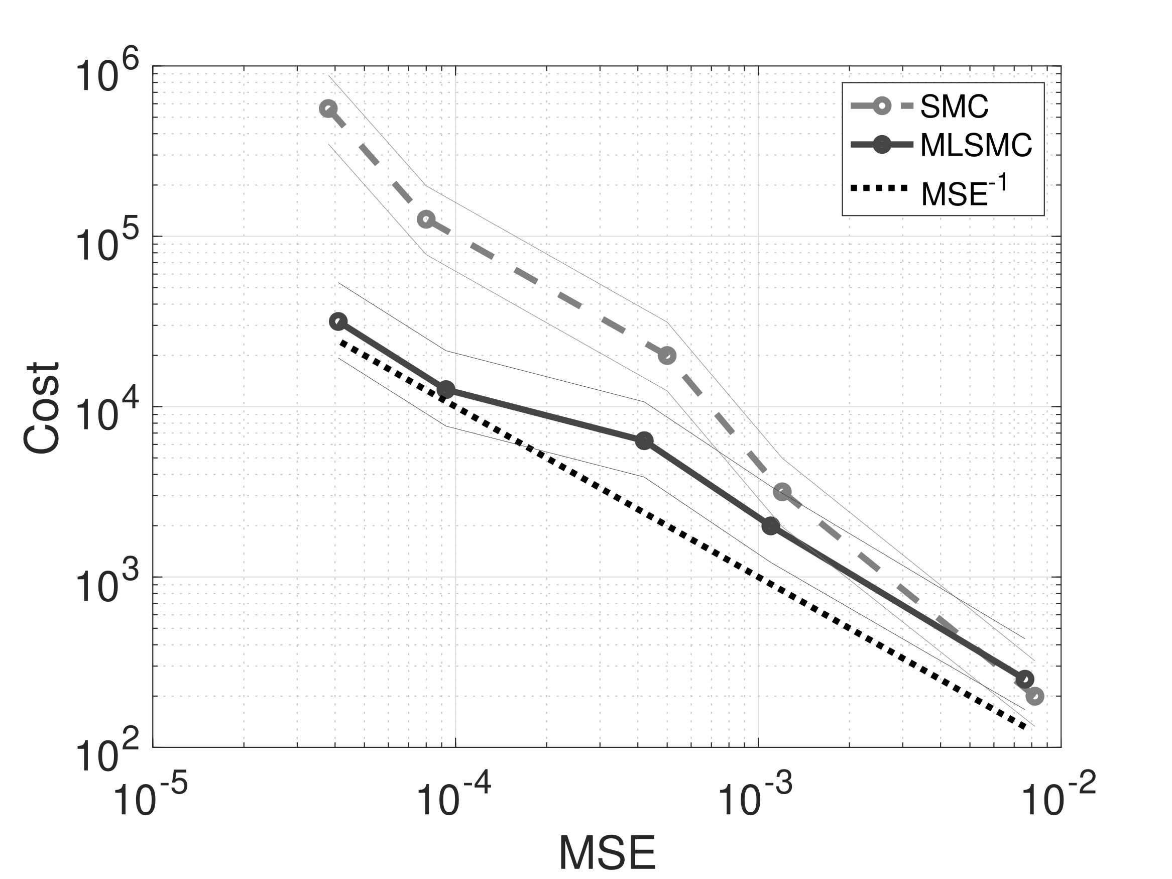
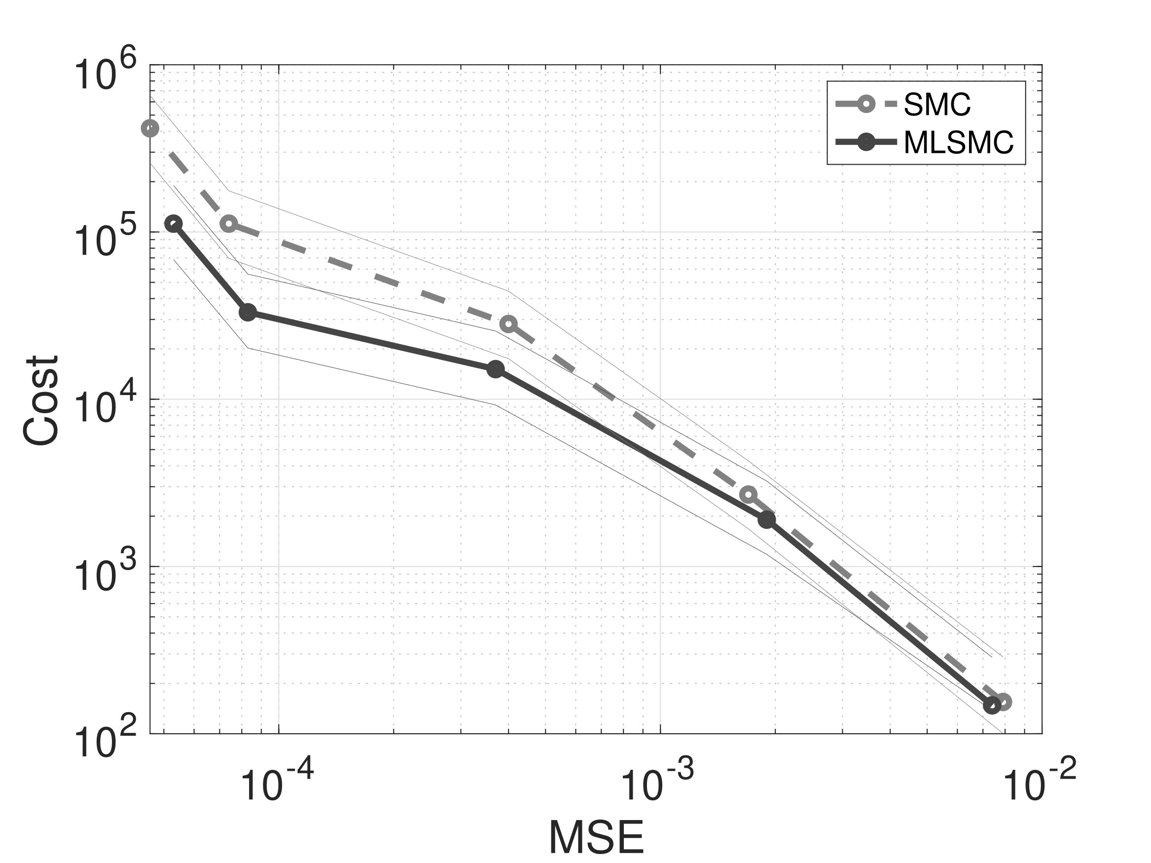
Figure 1:Regression problem: error vs cost plots for SMC and MLSMC using TNN priors. Left: . Right: . Credible intervals are provided by thin curves.
Binary MNIST Classification
As a second proof of concept, we consider a simplified binary MNIST LeCun et al., 2010 classification task using principal components (PCs) of the original image dataset, with . The results are similar to the regression case, and are presented in Figure Figure 2.
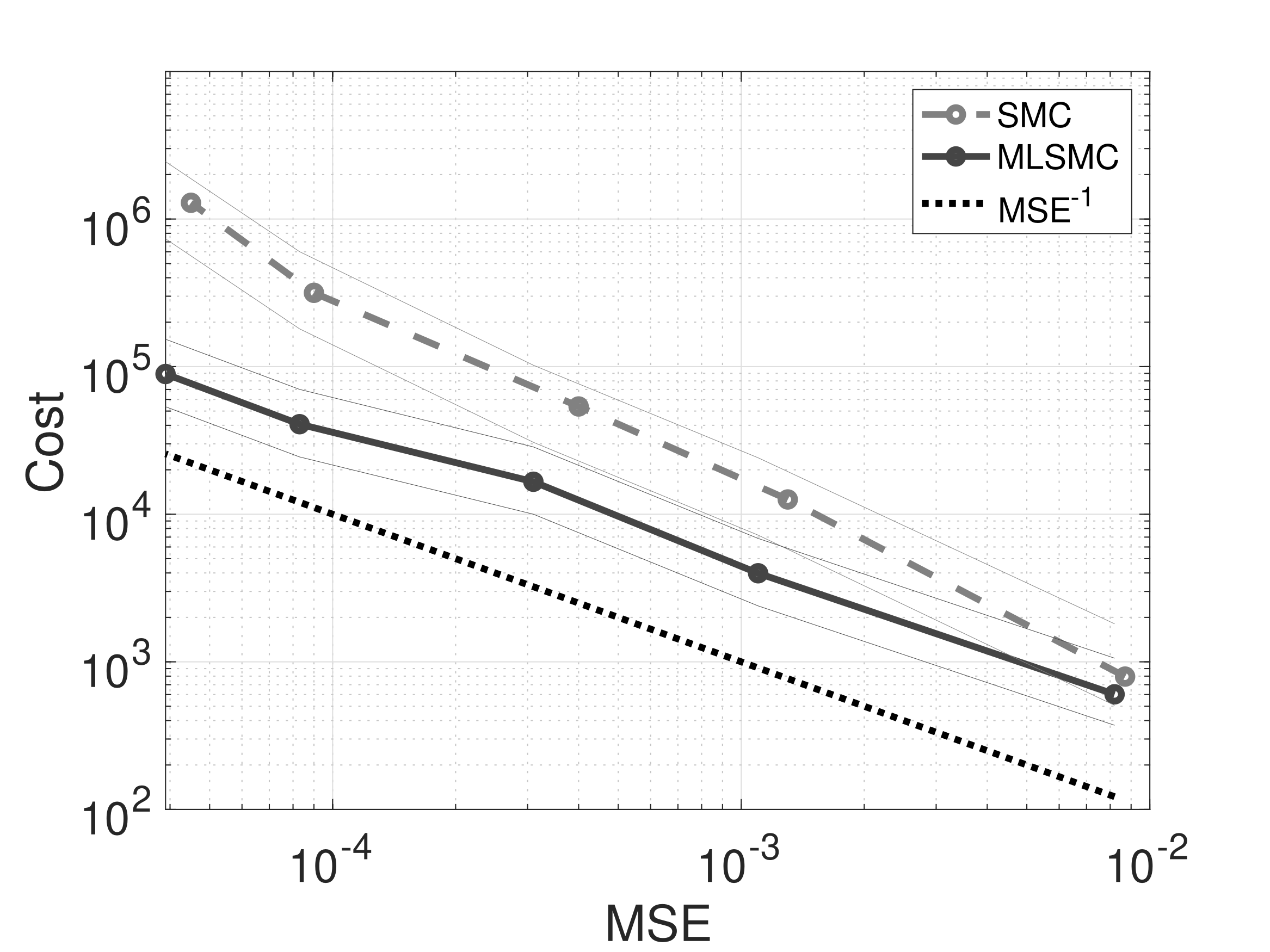
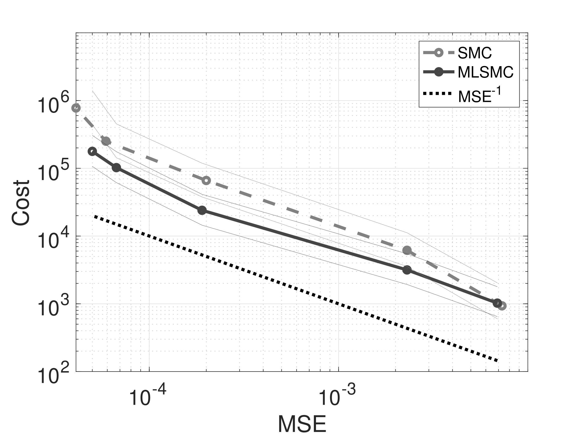
Figure 2:MNIST Classification problem: error vs cost plots for SMC and MLSMC, using TNN priors. Left: . Right: . Credible sets are provided in the thin curves.
Parallel SMC
For this section, we will assume a fixed and finite network architecture of the standard form, as introduced in Section Bayesian neural networks. This gives rise to a computable target distribution (up to a normalizing constant) .
A first source of parallelism is internal to a single SMC run: the MCMC mutation of each particle can proceed concurrently Lee et al., 2010Paige et al., 2014Syed et al., 2024, and it is in the mutations that the likelihood evaluations, the dominant computational cost, take place. Two hardware caveats apply. Each core must have sufficient memory available, or else the “memory wall” is hit Ivanov et al., 2021. Resampling forces communication among all particles, a potential bandwidth bottleneck, although on single-instruction-multiple-data (SIMD) hardware such as a single multi-core CPU or GPU this is usually benign. Being simple to implement, and sometimes exhibiting strong parallel scaling Lee et al., 2010, this intra-SMC parallelism is the most widely used.
Beyond this, one can run several SMC samplers at once and combine them, as studied in Vergé et al. (2015)Whiteley et al. (2016). The schemes recommended there typically make all samples communicate, which aids stability but works against scalability once a large model must be spread over many SIMD nodes whose inter-connect is slower, or absent altogether. In the island particle model Vergé et al., 2015, the total sample budget is divided into SMC islands of samples apiece. If the SMCs never interact and are combined by naive (equal-weight) averaging, an asymptotic bias penalty of order appears Crisan et al., 2018Vergé et al., 2015. However,* weighting each SMC appropriately removes this penalty* Whiteley et al., 2016Dai et al., 2022. The scalable parallel sampler that results is denoted SMC.
Algorithm 3 displays the SMC method, and we define the consistent (in , for finite suitably large) SMC ratio estimator as
This estimator is consistent, which is not the case for a naive unweighted average. See Proposition 3 and the discussion above.
Parallel MCMC
MCMC can also exploit parallel resources: one can retain a single sample from each of parallel chains, each run for warm-up epochs, achieving Margossian et al., 2025, which is indistinguishable from the single-chain result for , at a parallel cost equivalent to SMC when the integrated autocorrelation time matches the total number of mutation epochs. However, unlike SMC, the resulting estimator is not consistent for finite , which can potentially spoil convergence. A systematic empirical comparison of parallel SMC and parallel MCMC for Bayesian deep learning is given in Liang et al. (2024).
Theoretical Result
The convergence result is made rigorous in the following proposition. Suitable assumptions and proof are provided in Liang et al. (2025).
Numerical experiments
As above, we will measure wall-clock time complexity in terms of function evaluations, as an implementation and hardware agnostic proxy. We will refer to a likelihood evaluation as an epoch, in analogy with stochastic gradient descent (SGD) Robbins & Monro, 1951Bottou, 2010 based optimization methods like Adam Kingma & Ba, 2014. However, note that the time to compute an epoch of mini-batches depends heavily on the size of the problem and the details of the hardware and implementation. If all data fits on a single computational unit (either a node or a core), then a serial epoch of mini-batch likelihood computations will typically require much longer wall-clock time in comparison to a single likelihood evaluation. In contrast, if only a single mini-batch fits on a node, and interconnect is slow, then even data parallel may be slower than serial mini-batches. It is also worth noting that mini-batch gradients can deliver comparable gain to full gradient steps far from convergence, which can significantly accelerate progress as measured by epochs Bottou et al., 2018.
Proof of concept
First, we will consider logistic regression on the Australian Credit data Quinlan, 1987, illustrating comparable results to state-of-the-art (SOTA) parallel MC algorithms and the convergence guaranteed by Proposition 3.
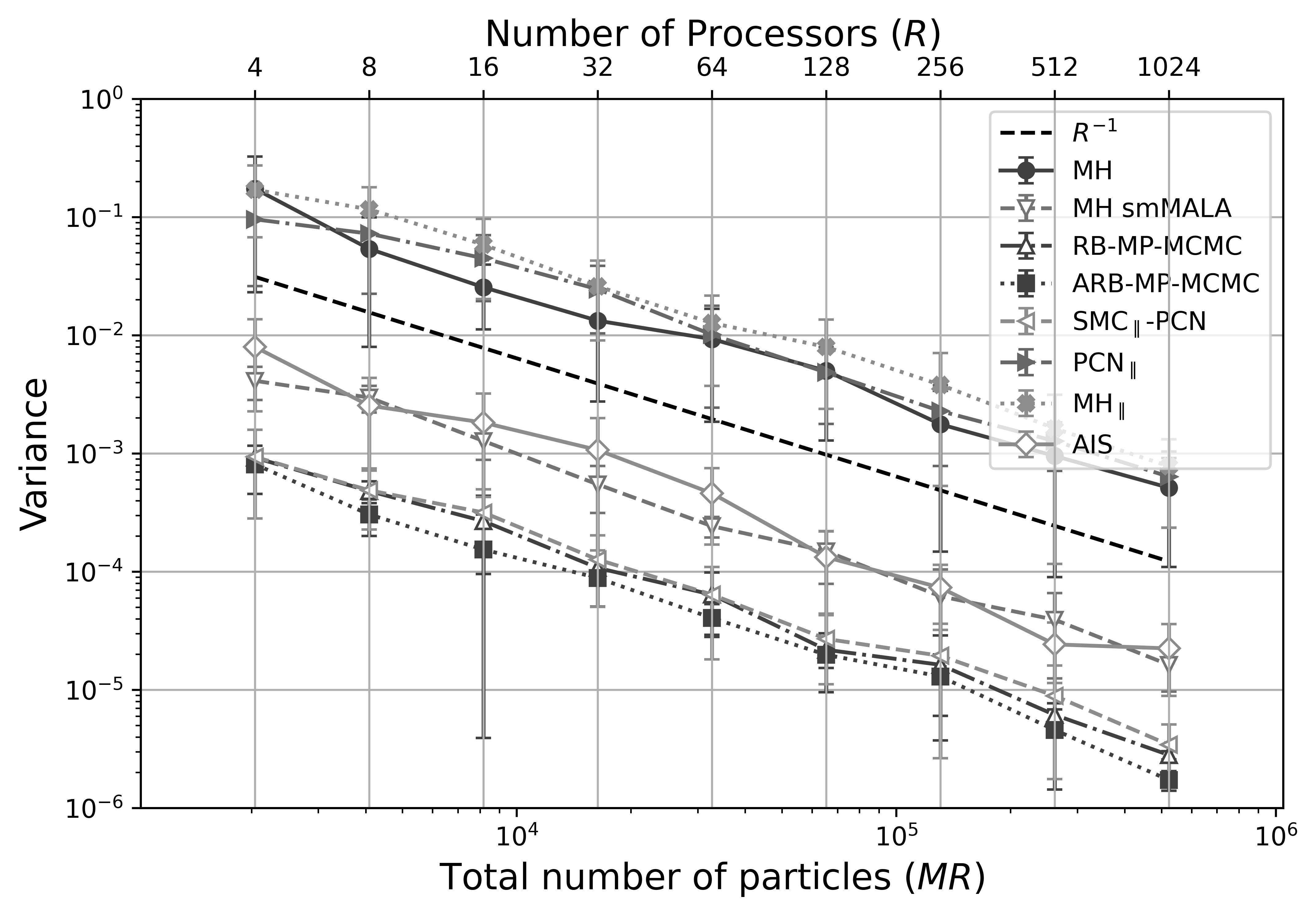
Figure 3:Empirical variance of posterior mean estimates for Bayesian logistic regression on Australian Credit (, ), for SMC-pCN, various MCMC methods, and AIS. SMC-pCN and the MCMC baselines are compared at matched total sample size , with particles per process; AIS is equivalent to particle per process. SMC-pCN uses pCN mutations with 30 mutation steps per tempering stage and adaptive tempering that keeps the effective sample size above . Curves are averaged over 25 repetitions; vertical bars show standard errors. Both axes are log-scaled. Some MCMC curves are reproduced directly from Schwedes & Calderhead (2021), with the authors’ permission.
The dataset has covariates and data and Bayesian logistic regression is used. We compare SMC-pCN (preconditioned Crank–Nicolson, pCN) with annealed importance sampling Neal, 2001, various MCMC methods, and recent synchronous-parallel MCMC Schwedes & Calderhead, 2021. Figure Figure 3 reports how the empirical variance of the posterior mean estimates decays with the number of samples and of parallel processes; the decay matches the rate of Proposition 3. Among the baselines in the figure that avoid communication scaling with , SMC-pCN achieves the lowest empirical variance. SMC and AIS incur a per-sample overhead in cost (, where are the mutations at tempering step ), but this is offset by intra-parallelism ().
IMDb dataset
We now consider a large problem in semantic classification of natural language, using the IMDb dataset Maas et al., 2011 of movie reviews, split evenly into training and test sets.
Architecture. Each review is mapped to a fixed feature vector by SBERT embeddings Reimers & Gurevych, 2019 from the model all-mpnet-base-v2 Song et al., 2020[2], whose weights are frozen throughout: they are used only to produce the 768 dimensional [CLS] embedding and are never sampled. On top of these embeddings we place (i) one hidden layer with 128 neurons, (ii) ReLU activation, (iii) a final linear layer, and (iv) a softmax output. Inference is over* all* weights and biases of this network, of dimension , and not merely the final classifier head. The whole train (25000 data) and test dataset (25000 data) are considered.
Sampling setup. The likelihood is the softmax (categorical cross-entropy) likelihood over the whole training set of 25000 reviews, and inference uses an adaptive likelihood-tempering SMC sampler with HMC mutations of length . We compare SMC against two baselines that share the same prior, likelihood, and frozen embeddings: HMC, which averages over independent HMC chains of length , and a single serial HMC run of length ; in every method the HMC step size is adapted to a common acceptance-rate target, so the comparison is made at matched cost.
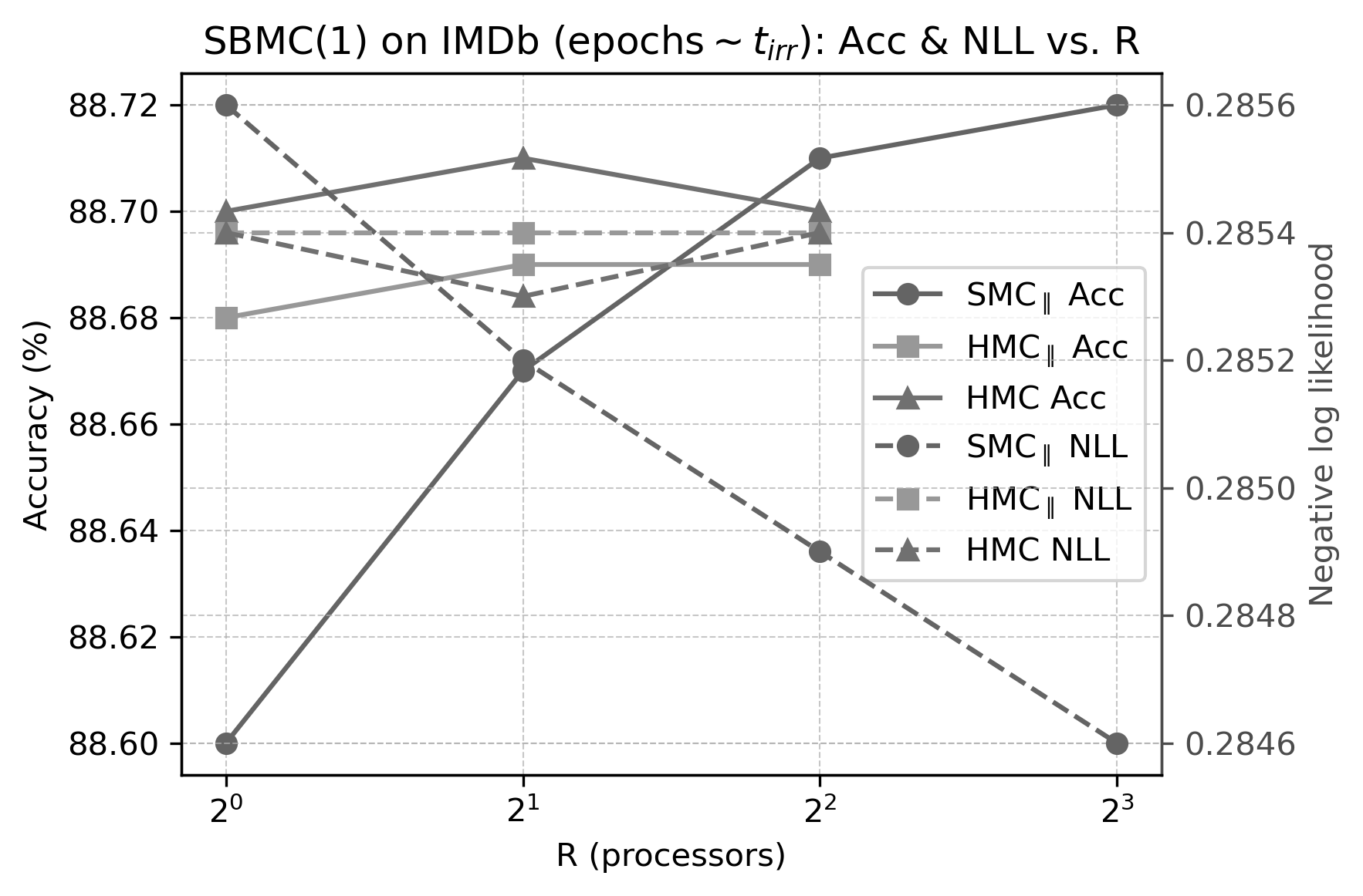
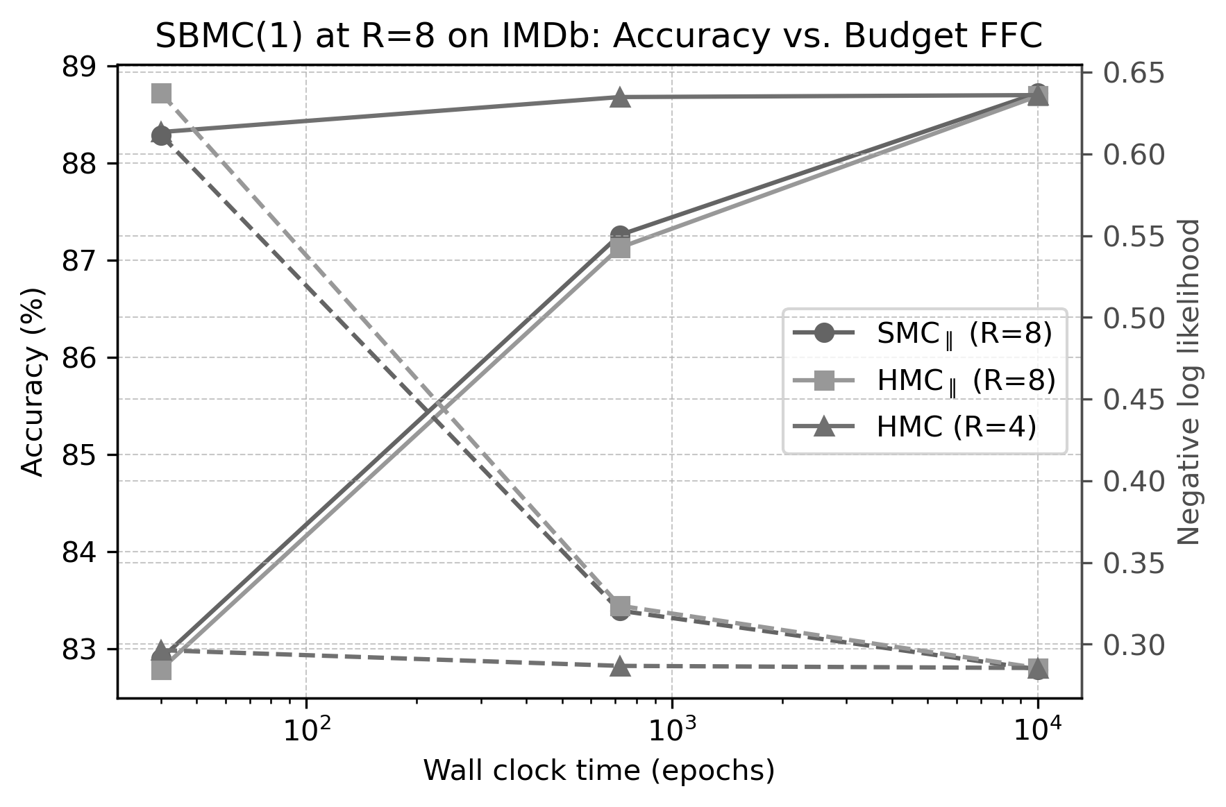
Figure 4:IMDb sentiment classification, with the full posterior over all network weights, using SMC with particles for each of SMC runs, HMC mutations, and adaptive tempering that keeps the effective sample size above . Left: test accuracy and negative log-likelihood (NLL) against the number of parallel runs at a budget of about epochs, alongside a serial HMC baseline given epochs and HMC with chains with epochs each. Right: converged values () showing the catastrophic failure (collapsed accuracy and inflated NLL) once the budget drops below . The - and budget-axes are log-scaled; all curves are averaged over 5 realizations.
Experiment. Denote by the number of evaluations of per mutation step, which we refer to as epochs, and by the number of tempering-and-mutation steps. The product (or for an adaptive schedule) is the total simulation cost, which we call the* irreducible serial time* : the serial simulation the sampler needs in order to mix, which cannot be removed by adding more parallel runs. In practice is read off empirically as the budget at which accuracy and NLL plateau, here epochs. When and/or are too small, so that the budget falls well short of , the sampler has not mixed and the method* catastrophically fails*: test accuracy collapses and NLL inflates. Figure Figure 4 summarises this behaviour. The left panel shows performance as a function of at , where SMC improves steadily with and matches the far more expensive serial HMC baseline; the right panel fixes and reduces the budget below , exposing the catastrophic failure of SMC and HMC once the budget falls short of the irreducible time.
Parts of this chapter are adapted from Chada et al. (2025), Liang et al. (2025), and Liang et al. (2024).
- Doucet, A., De Freitas, N., & Gordon, N. J. (Eds.). (2001). Sequential Monte Carlo methods in practice. Springer.
- Doucet, A., & Johansen, A. M. (2011). A tutorial on particle filtering and smoothing: fifteen years later. In D. Crisan & B. Rozovskii (Eds.), The Oxford Handbook of Nonlinear Filtering (pp. 656–704). Oxford University Press.
- Del Moral, P., Doucet, A., & Jasra, A. (2006). Sequential Monte Carlo samplers. Journal of the Royal Statistical Society: Series B (Statistical Methodology), 68(3), 411–436.
- Geyer, C. J. (1991). Markov chain Monte Carlo maximum likelihood. Computing Science and Statistics: Proceedings of the 23rd Symposium on the Interface, 156–163.
- Gelman, A., & Meng, X.-L. (1998). Simulating normalizing constants: from importance sampling to bridge sampling to path sampling. Statistical Science, 13(2), 163–185.
- Neal, R. M. (2001). Annealed importance sampling. Statistics and Computing, 11(2), 125–139.
- Chopin, N. (2002). A sequential particle filter method for static models. Biometrika, 89(3), 539–552.
- Beskos, A., Jasra, A., Law, K., Tempone, R., & Zhou, Y. (2017). Multilevel sequential Monte Carlo samplers. Stochastic Processes and Their Applications, 127(5), 1417–1440.
- Beskos, A., Jasra, A., Law, K., Marzouk, Y., & Zhou, Y. (2018). Multilevel Sequential Monte Carlo with Dimension-Independent Likelihood-Informed Proposals. SIAM/ASA Journal on Uncertainty Quantification, 6(2), 762–786.
- Vergé, C., Dubarry, C., Del Moral, P., & Moulines, E. (2015). On parallel implementation of sequential Monte Carlo methods: the island particle model. Statistics and Computing, 25(2), 243–260.
- Whiteley, N., Lee, A., & Heine, K. (2016). On the role of interaction in sequential Monte Carlo algorithms. Bernoulli, 22(1), 494–529.
- Liang, X., Lukens, J. M., Lohani, S., Kirby, B. T., Searles, T. A., Qiu, X., & Law, K. J. H. (2025). Scalable Bayesian Monte Carlo: fast uncertainty estimation beyond deep ensembles.
- Sell, T., & Singh, S. S. (2023). Trace-class Gaussian priors for Bayesian learning of neural networks with MCMC. Journal of the Royal Statistical Society Series B: Statistical Methodology, 85(1), 46–66.
- Chada, N. K., Jasra, A., Law, K. J. H., & Singh, S. S. (2025). Bayesian deep learning with multilevel trace-class neural networks. SIAM Journal on Mathematics of Data Science, 7(3), 1210–1240.
- Dai, C., Heng, J., Jacob, P. E., & Whiteley, N. (2022). An Invitation to Sequential Monte Carlo Samplers. Journal of the American Statistical Association, 117(539), 1587–1600.